1. Mini-Game Containers and Game Engines
A mini-game container can be thought of as a specialized WebView. On the rendering side, it strips away unnecessary DOM elements and keeps only Canvas. On the scripting side, it aligns with the ECMA-262 standard through JS polyfills or container bindings. Beyond that, the container must provide script loading and execution, WASM support, and multimedia capabilities like Audio and Video — all exposed to the JS layer via JSBinding, wrapped into BOM-style interfaces.
The reason mini-game containers are designed to comply with web standards is compatibility: this lets different game engines plug in without modification. The core idea is to standardize and unify underlying platform capabilities, shielding hardware and OS fragmentation inside the container, and exposing only a single programming model similar to the browser’s BOM/DOM. This allows engines like Cocos, Egret, Laya, and Unity WebGL to treat the container as a web runtime — no need for each engine to adapt to each platform’s native APIs. It’s essentially a local, lightweight re-evolution of WebView: the mini-game container is approximately a lightweight browser kernel.
In this model, the container handles platform standardization, and the engine handles content ecosystem. For example:
Container responsibilities:
- Provide a unified rendering context (Canvas/WebGL).
- Provide a unified script runtime (JS/WASM).
- Provide standardized input, audio, video, and multimedia APIs.
- Provide platform capability wrappers: networking, storage, payment, sharing, ads.
- Interface with the security sandbox, permission management, and performance isolation layers.
Game engine responsibilities:
- Provide high-level abstractions for scene management, physics, animation, and asset management.
- Provide developer-friendly editors and debugging toolchains.
- Provide a cross-platform, component-based development paradigm (UI, skeletal animation, particle systems, etc.).
- Manage game lifecycle, state synchronization, and rendering scheduling.
This article uses the Cocos engine rendering pipeline as a case study to walk through how a mini-game container loads assets and renders game components.
2. The Three Major Loops in a Game Engine
The game engine rendering pipeline is driven by three major loops: the Render Loop, the Event Loop, and the Game Loop. Here is an overview of all three:
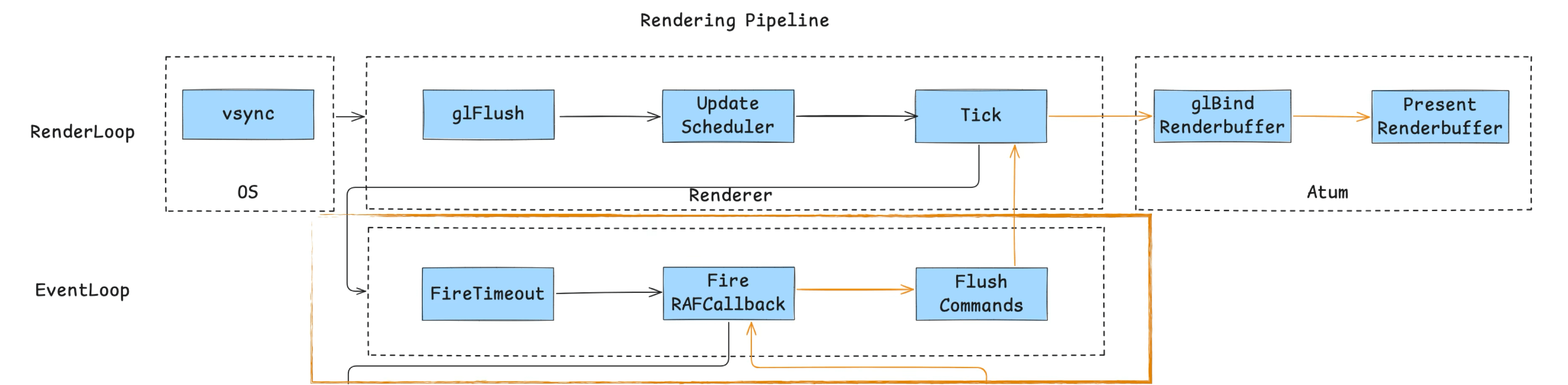
2.1 RenderLoop
The render loop is first. Its main flow looks like this:
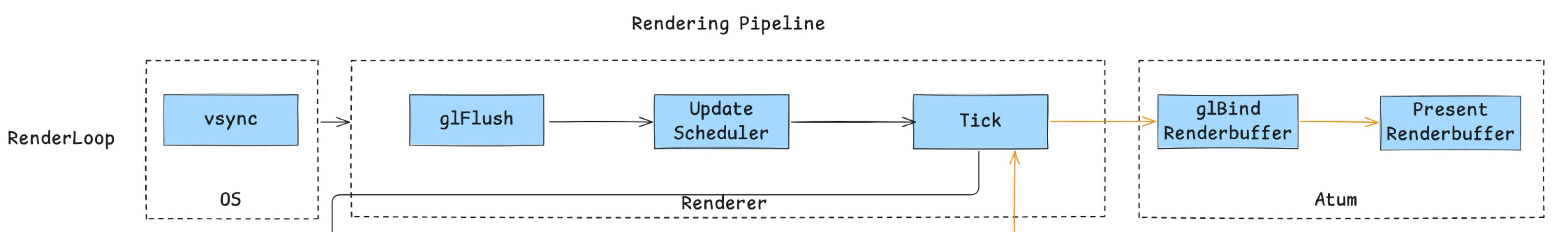
The entire render loop is driven by the system’s Vsync signal. On iOS, this originates from CADisplayLink, running rendering tasks through the main thread’s RunLoop, with frame rate control capabilities — on iOS you can set 30/60/90/120 FPS.
On the engine side, the core loop does three things each frame:
glFlush— flush GL command buffer: forces any queued OpenGL commands from the previous frame to execute, ensuring display memory and framebuffer data are consistent and preventing “frame delay” or stuttering from command backlog.UpdateScheduler— async task scheduling: dispatches async tasks scheduled for the current frame, such as audio callbacks and network event responses. This decouples non-rendering logic (like data updates) from the rendering path, improving main-thread concurrency.Tick— drive JS layer logic: every frame, via Binding, calls the JS-side Tick method to execute animations and state updates related to rendering. This decouples the logic layer from the render layer and improves cross-platform adaptability.
On the container side, iOS uses CAEAGLLayer to get GL commands onto screen in two steps:
glBindRenderbuffer— binds the current frame’s render result to the RenderBuffer, which serves as the on-screen buffer.PresentRenderbuffer— presents the RenderBuffer content to the screen, producing the final visible image.
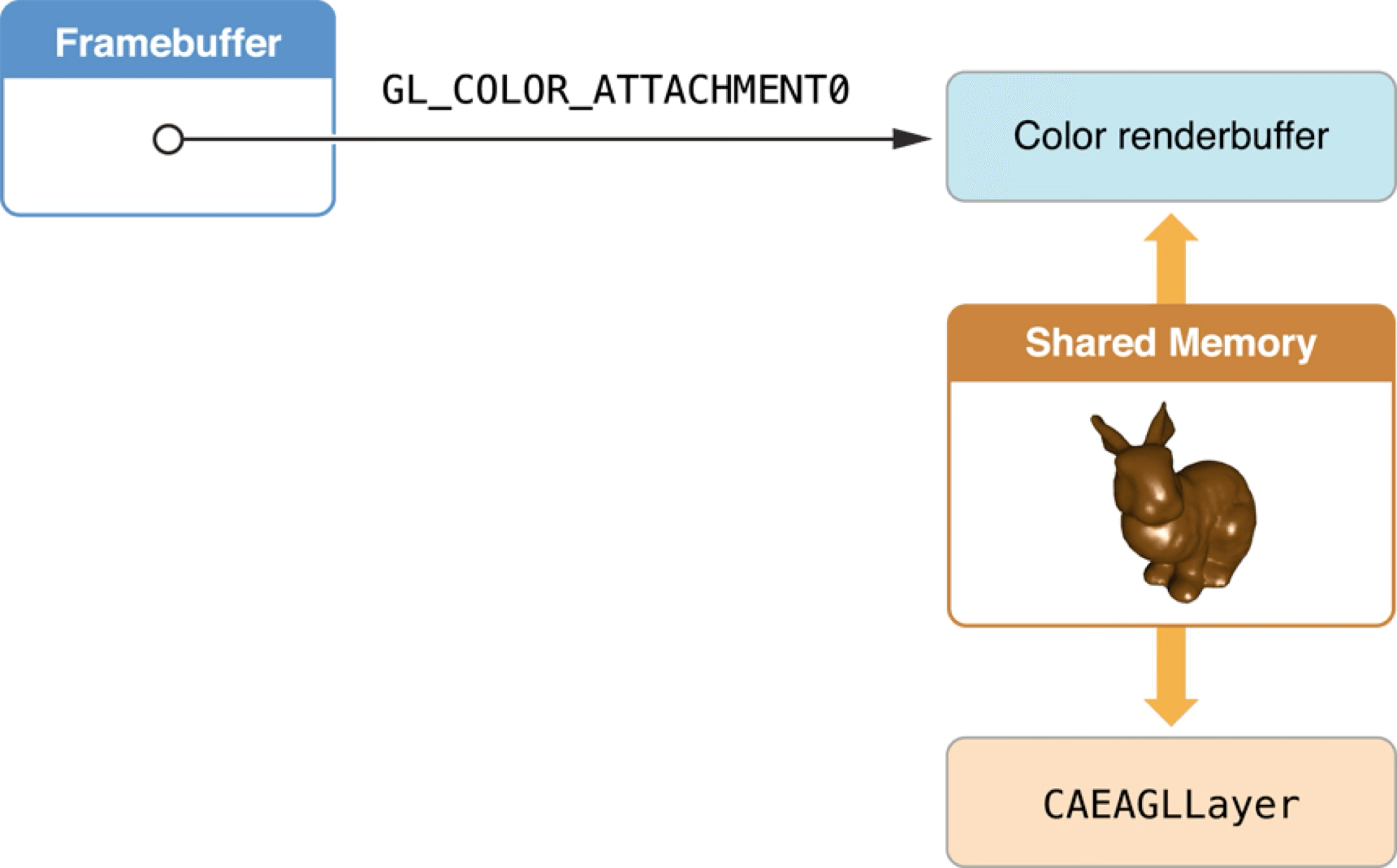
In iOS’s rendering architecture, CAEAGLLayer is the component ultimately responsible for display. As part of the Layer Tree, it directly references the shared-memory render buffer (Renderbuffer data). The system Compositor then composites CAEAGLLayer’s content with other UI elements (UIKit, SwiftUI) and outputs the final frame.
In each frame’s Tick task, JavaScript works with the game engine to produce the Framebuffer for that frame (covered in sections 3.5–3.10). Core Animation and OpenGL ES synchronize through the shared render buffer. This means the OpenGL render result is essentially just one canvas in the Layer Tree — it still needs to be composited with the system UI layer to produce the final display image.
Note: this article’s mini-game container uses OpenGL as its rendering backend only. With the rise of Metal, Vulkan, and other next-generation graphics APIs, RenderBuffer binding and on-screen presentation are moving toward a “parallel rendering + async display” model, improving smoothness and reducing latency at high frame rates.
The render loop runs synchronously, so if a frame’s logic doesn’t complete within 16.6ms at 60 FPS, it causes jank.
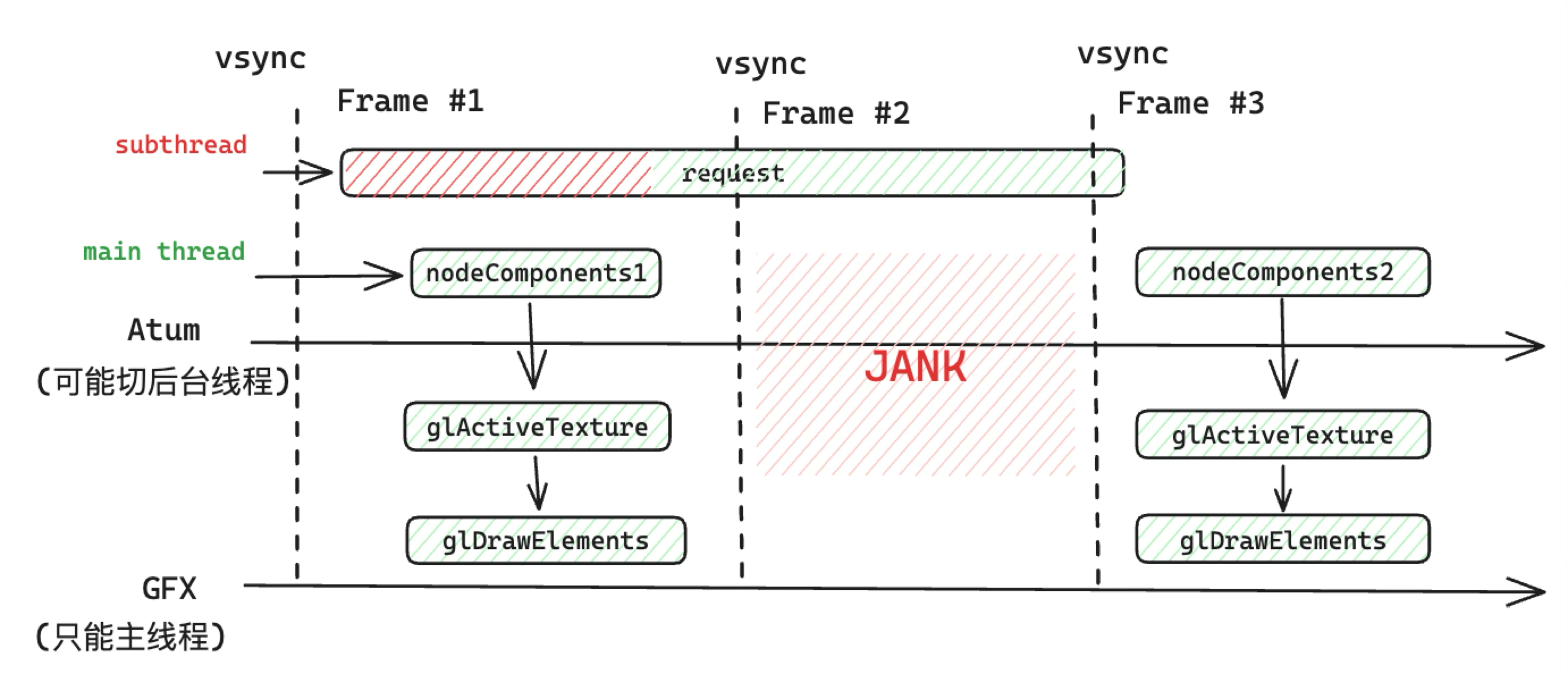
For example, in this bad case, running a Tick task with 136ms of JS execution on the main thread caused game animation stutter:
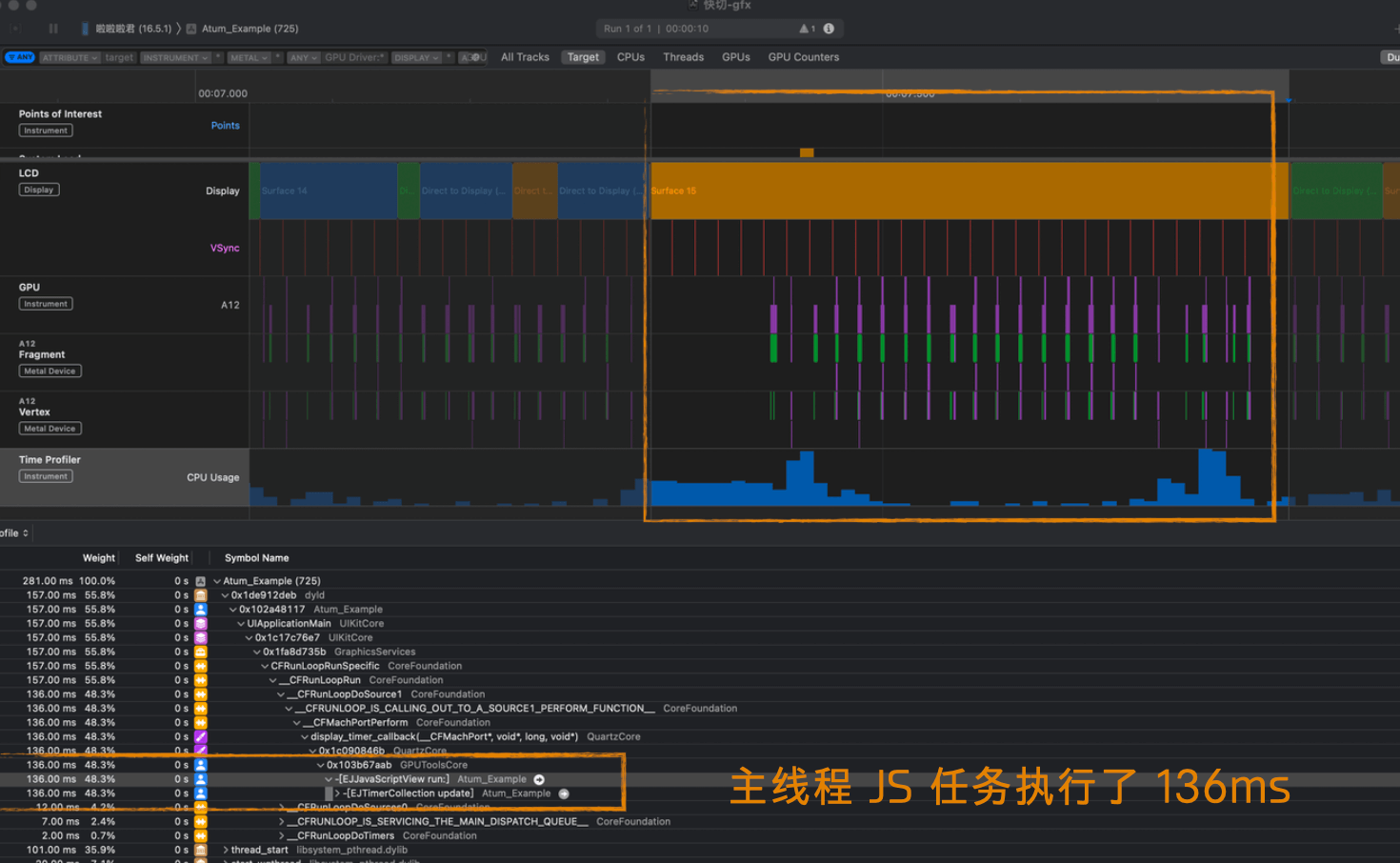
To keep the game running smoothly, you need to continuously optimize performance and minimize synchronous task latency. Profiling tools are essential — here are some commonly used ones:
- Xcode GPU Frame Debugger: An iOS graphics debugging tool for deep analysis of render pipeline bottlenecks, especially useful for Metal and OpenGL ES.
- RenderDoc: A mainstream cross-platform graphics debugging tool; captures frame data and analyzes resource and performance bottlenecks across pipeline stages. Supports OpenGL, Vulkan, DirectX, and more.
- inspector.js: Usable in web contexts; useful for analyzing DrawCalls, shaders, and resource bindings in WebGL scenarios.
- Mali Offline Shader Compiler: https://zhuanlan.zhihu.com/p/161761815 — An offline shader compilation and analysis tool for ARM Mali GPUs, used to evaluate shader complexity and instruction cost to optimize mobile rendering.
- Snapdragon Profiler: A frame capture tool that tracks Heavy DrawCalls and Overdraw, helping identify rendering bottlenecks and redundant computation.
2.2 EventLoop
Going deeper, from the Tick task we enter the second loop — the Event Loop.
Because the mini-game container is not a WebView — it only has a JS engine — we need to implement an event loop mechanism to drive JS execution (it doesn’t need to fully align with the browser standard, just satisfy container requirements). As the diagram shows, it consists of three main tasks:
- Consume macrotasks (timers, etc.): process tasks registered via
setTimeout,setInterval, etc., ensuring timers fire correctly. - Consume rAF tasks: this primarily drives GameLoop logic. The game’s main loop is typically mounted in an rAF callback, updating rendering and logic frame by frame.
- Flush current-frame Commands: execute render commands and queued interface update instructions, completing the current frame’s render cycle.
A closer look at the rAF implementation is worth it. Early on, rAF was simulated with setTimeout(0), with this call chain:
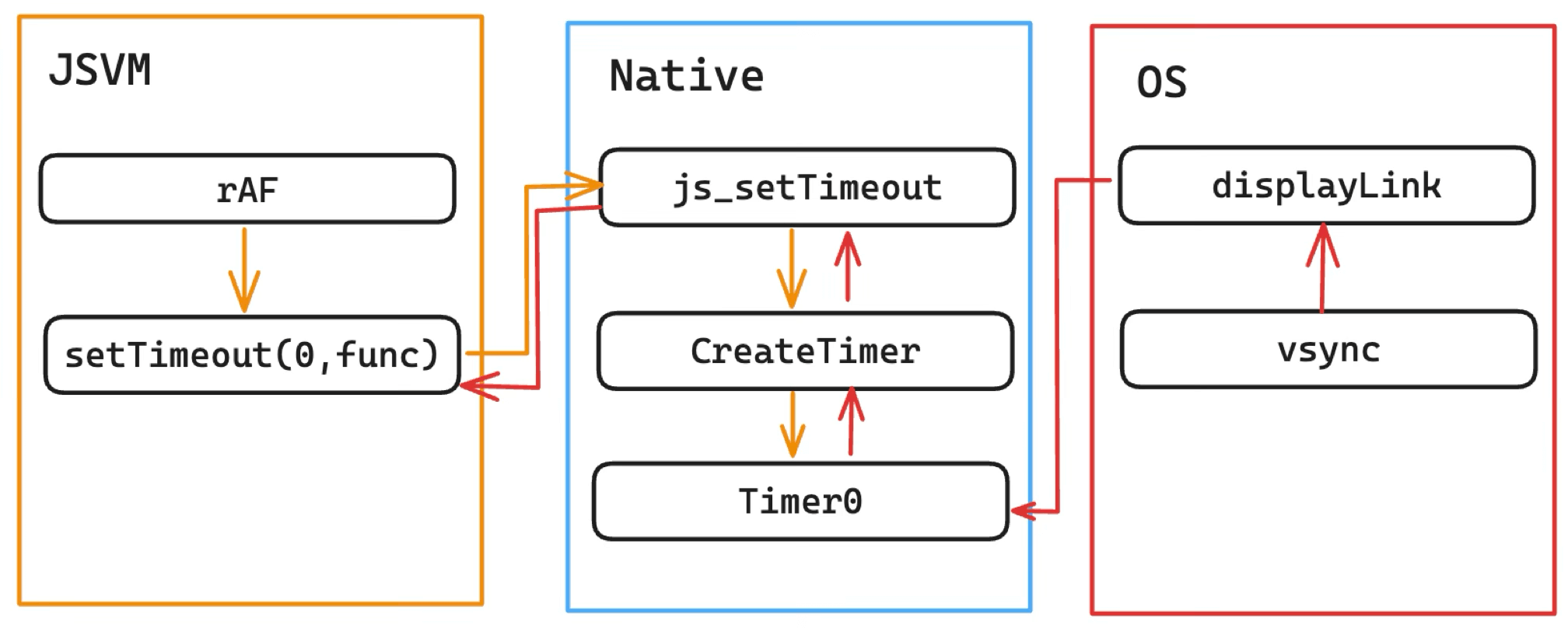
This approach had problems:
- Non-standard: simulated with
setTimeout(0)rather than driven directly by vsync. - Long chain: Native maintained the Timer queue and would call back to JS only after consuming the vsync signal.
It was later refactored to follow the WHATWG standard:
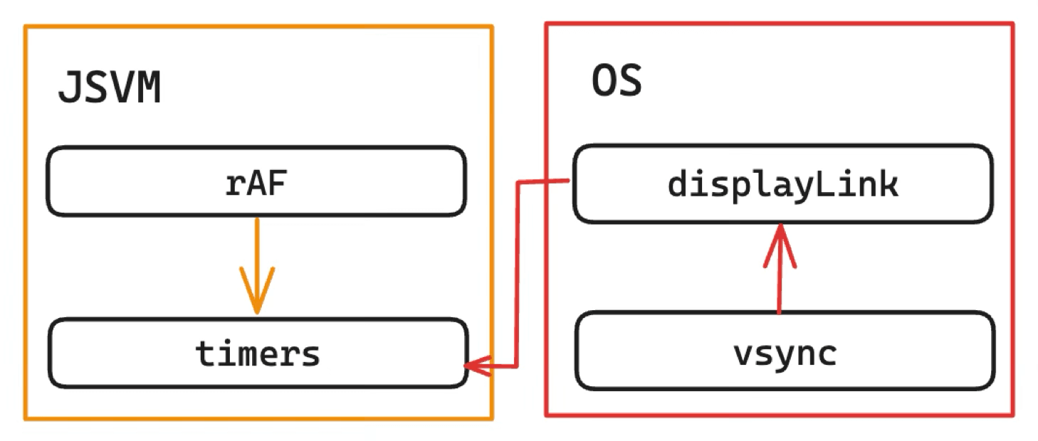
Benefits:
- Standardized: JS is called directly after vsync.
- Lower overhead: JS maintains the Timers queue, eliminating the JSBinding call overhead of the native intermediary.
This illustrates how rendering performance optimization lives in implementation details — it takes digging and refinement.
Through this event loop, the container maintains coordinated operation between the JS engine and the rendering system, keeping the game running and updating continuously.
2.3 GameLoop
The GameLoop expands into Chapter 3 — the life of a game component:
Before unrolling the full picture, here’s the traditional rendering pipeline for a mini-game container using OpenGL as its rendering backend:
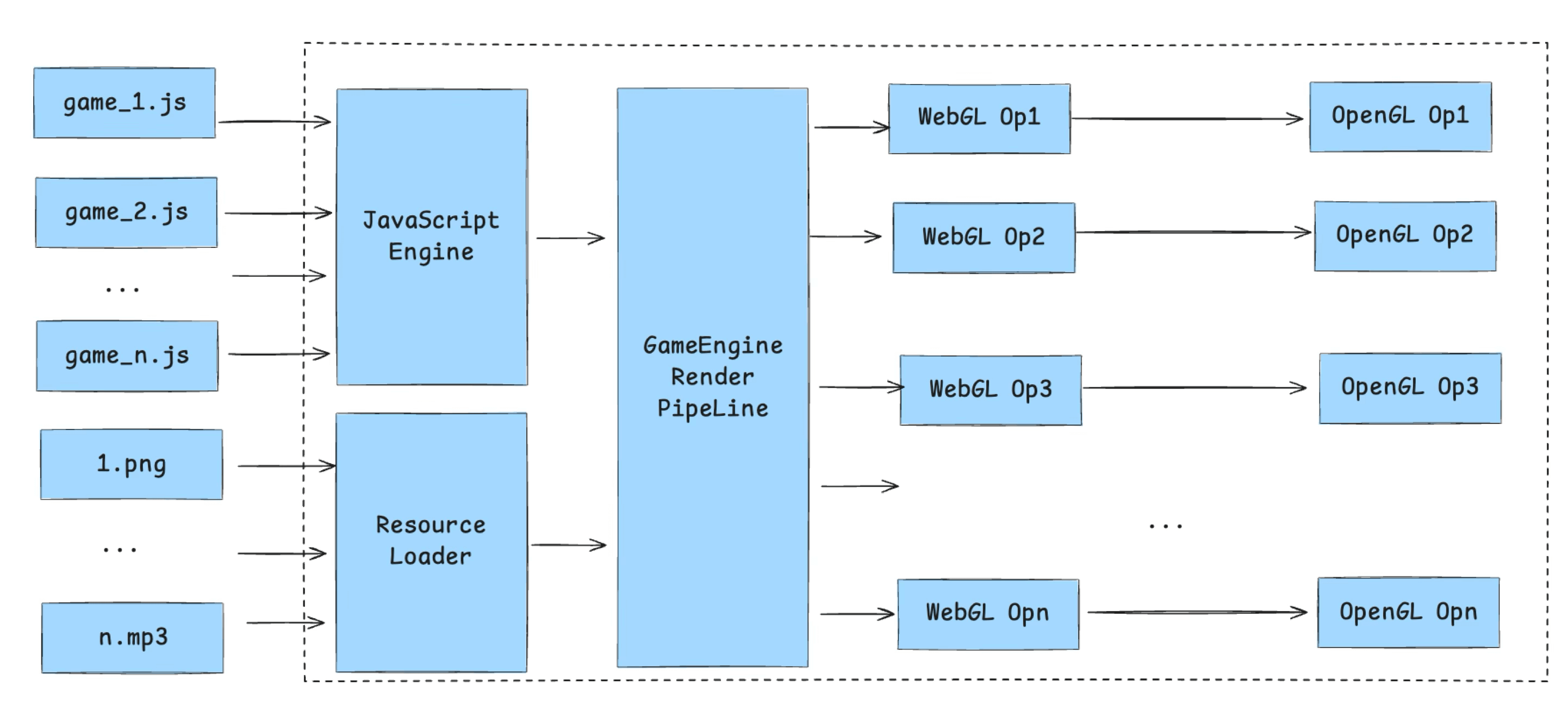
First comes asset loading, which involves two completely different resource types — script assets and static assets. Script assets are handled by the JS Runtime; static assets each have their own handling depending on type — images, fonts, audio, video, and the special case of skeletal animation. Since this article focuses on rendering, we won’t expand on the asset loading pipeline.
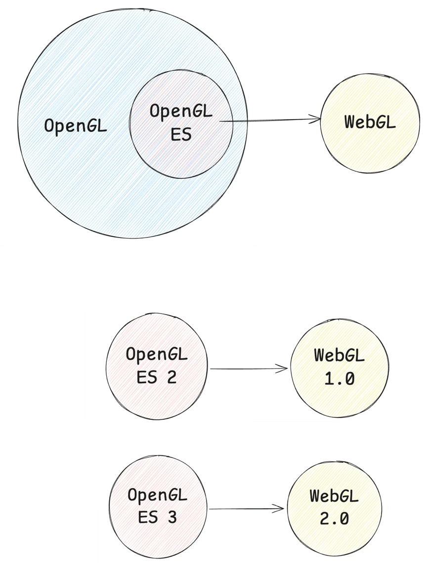
These assets are then processed by the game engine’s rendering pipeline. JS drives the generation of WebGL commands, which go through JS Binding and ultimately call into C++ or native-side OpenGL instructions — WebGL is a subset of OpenGL, so there’s a one-to-one correspondence.
This process often produces rendering bottlenecks. The main hardware resources to monitor are CPU, GPU, and bandwidth. On today’s resource-constrained mobile hardware, game optimization becomes an art of balance — when a bottleneck can’t be eliminated, it needs to be shifted. A common example is moving bottlenecks from CPU to GPU using Compute Shaders, GPU skinning, Animation Baking, GPU particles, etc.
CPU is the most common bottleneck. Rather than covering business-side optimizations (Culling, Batching to reduce DrawCalls), here are some container-side optimization approaches:
- JSBinding calls can create bottlenecks — one approach is batching: batching call counts with CommandBuffer to increase throughput, and merging call implementations with high-level graphics libraries like GFX.
- Synchronous JS tasks that block the main thread can be moved to Native for compute-intensive work.
- For JS interpretation overhead, consider JIT or WASM.
- GC is also an area with room for optimization.
GPU bottlenecks generally stem from overly complex Fragment Shaders, or oversized Vertex Buffers (e.g., triangle counts exceeding thresholds — typically 500K–1.5M triangles on mobile). High Overdraw also causes the GPU to do a lot of unnecessary work.
Bandwidth bottlenecks are primarily addressed with texture compression (desktop can also use deferred rendering and post-processing). A rule of thumb from the community:
If your game runs at 60 fps, each frame has roughly 2*1024/60 = 34 MB of bandwidth. If your GBuffer resolution is 1280×1080, writing one GBuffer (RGBA, 4 bytes) costs 1280*1080*4/1024/1024 = 5.2 MB. Three GBuffers = 15.6 MB.
Assuming a reasonable Overdraw of 1.5x, that’s 15.6 × 1.5 = 23.4 MB. Add scene, UI, and character rendering on top of that, and you easily exceed the recommended 34 MB/frame budget.
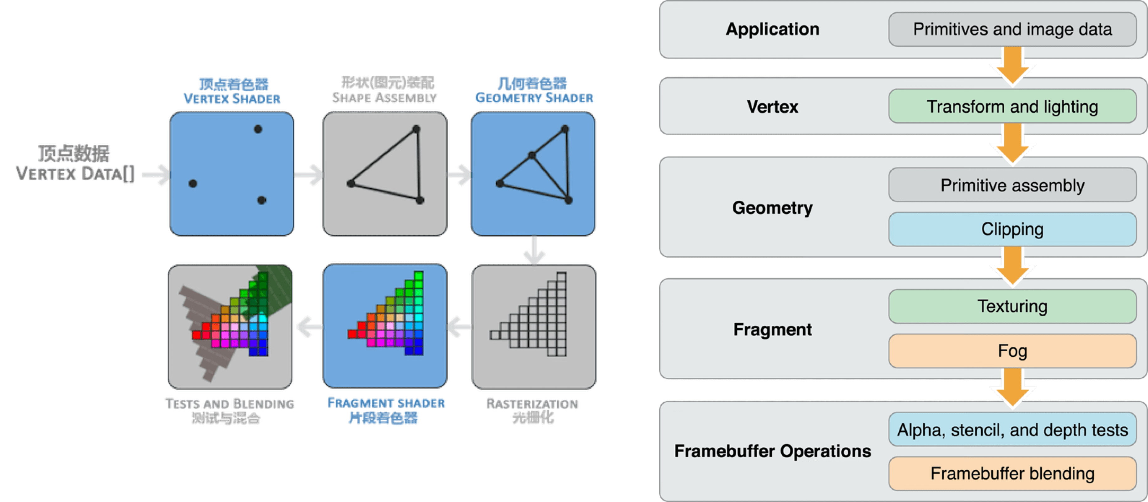
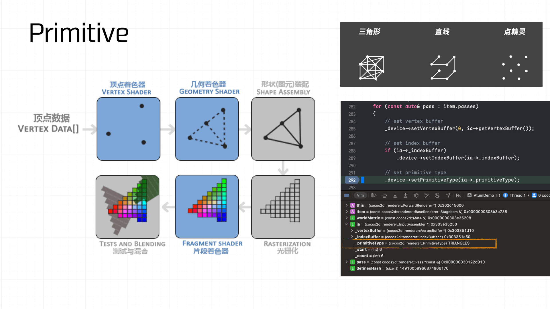
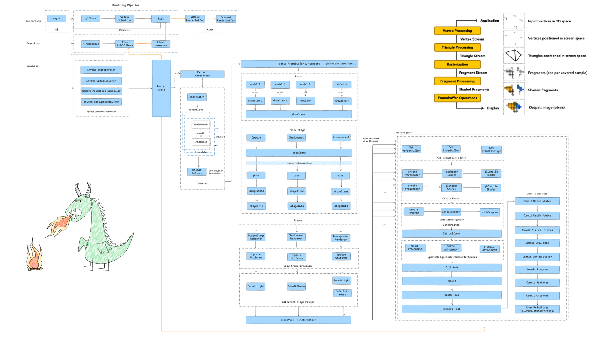
Here’s a typical synchronous rendering pipeline:
- Application layer provides vertex data.
- Vertex shader normalizes the vertices.
- Primitive assembly builds geometric primitives.
- Rasterization discretizes primitives into fragments, each corresponding to a pixel area on screen.
- Fragment shader executes texture sampling, color calculation, fog effects, and other per-pixel processing.
- Testing and blending operations (Alpha, depth, stencil tests) run, and results are written to the Framebuffer.
Once the Framebuffer is built, we return to the CAEAGLLayer on-screen presentation described in section 2.1.
Now let’s unroll the full picture and follow a game component through its entire life.
3. The Life of a Game Component
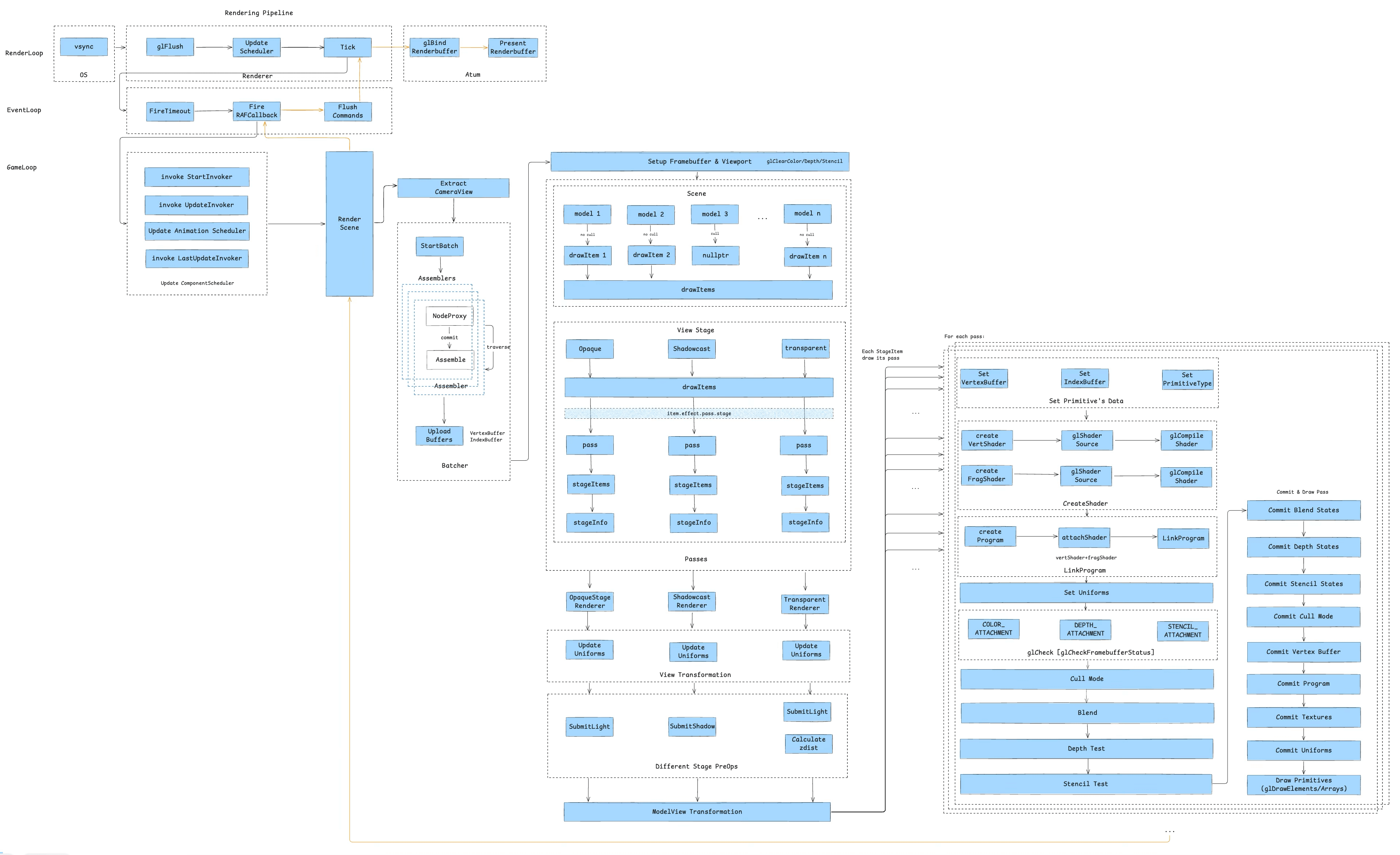
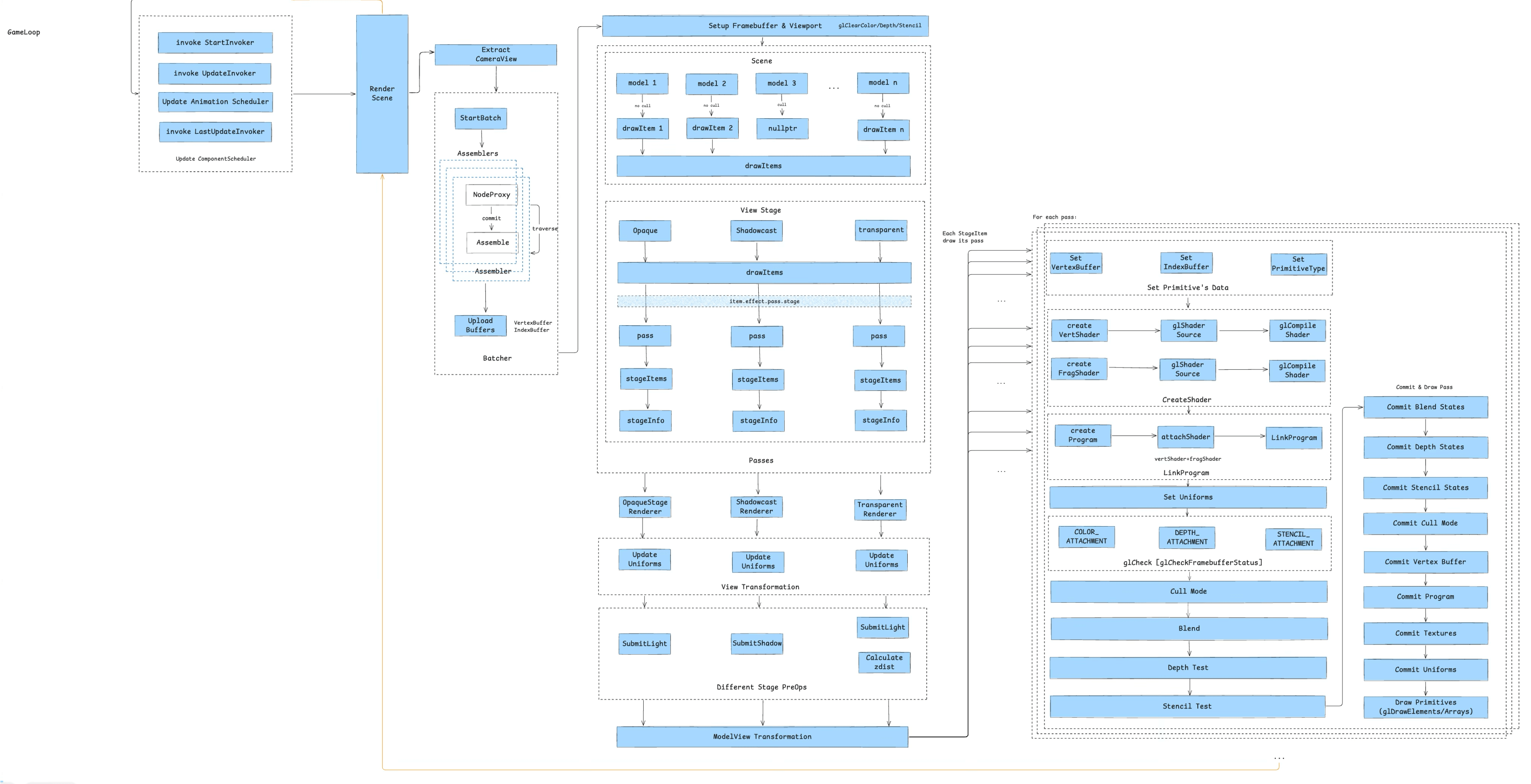
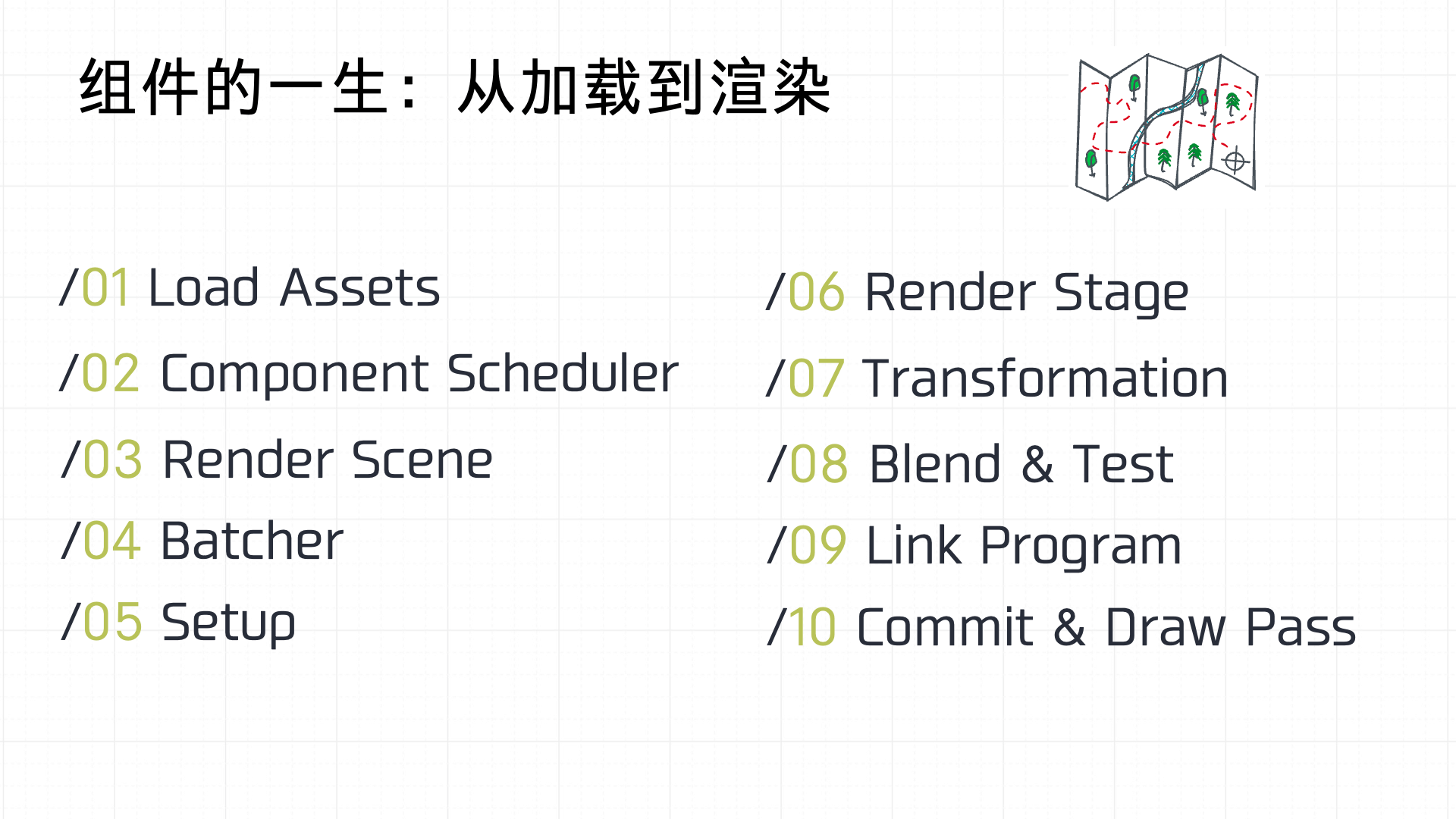
Here’s the full diagram of a game component’s journey from load to screen:
This pipeline can be broken into 10 stages:
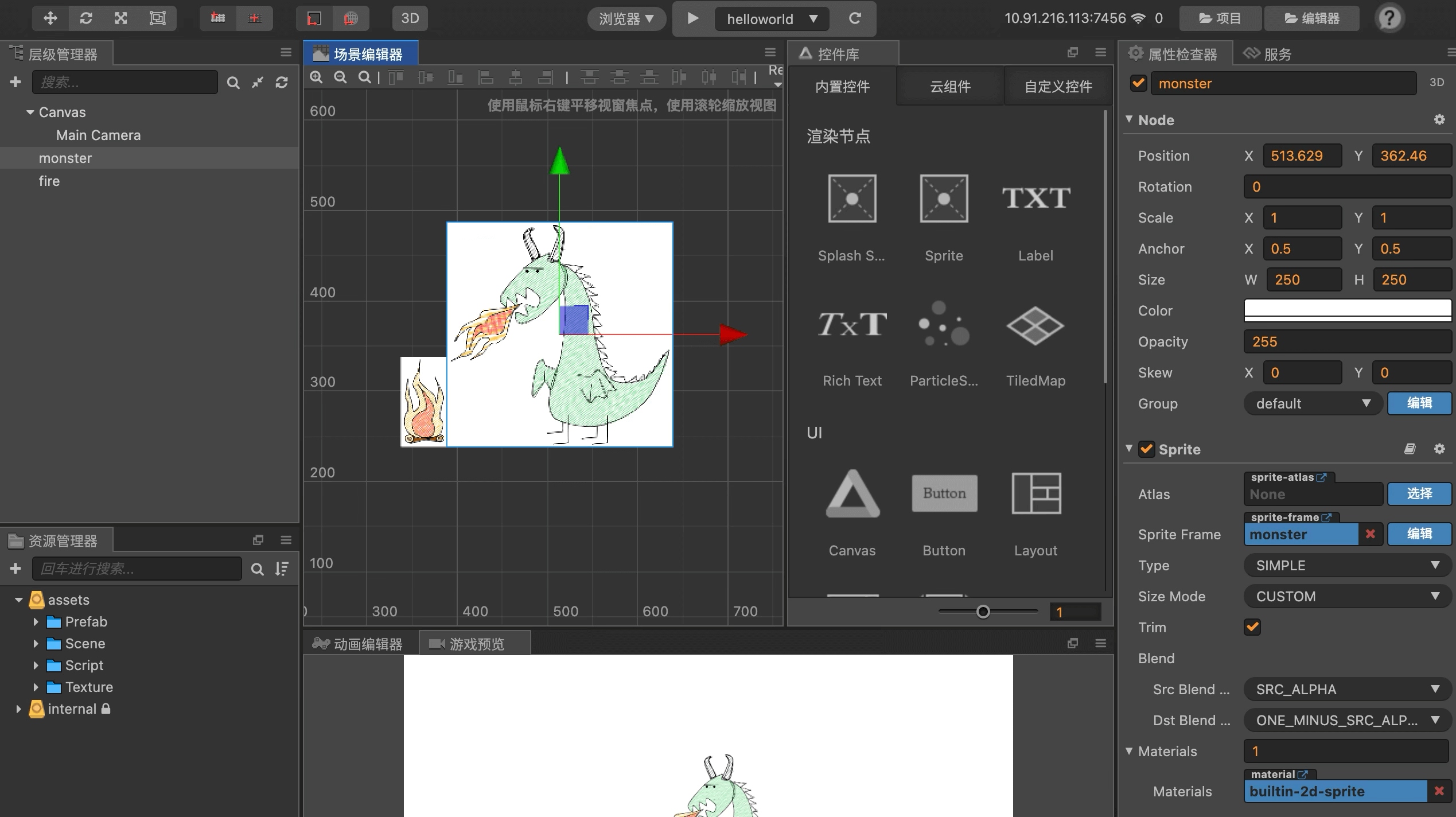
To make this concrete, I prepared a minimal Cocos game demo. Here’s the scene:
And here’s the main scene code:
`const { ccclass } = cc._decorator;
@ccclass export default class Helloworld extends cc.Component {
protected onLoad(): void {
    console.log('onLoad');
}

start () {
    console.log('Hello World');
}
} `
3.1 Load Assets
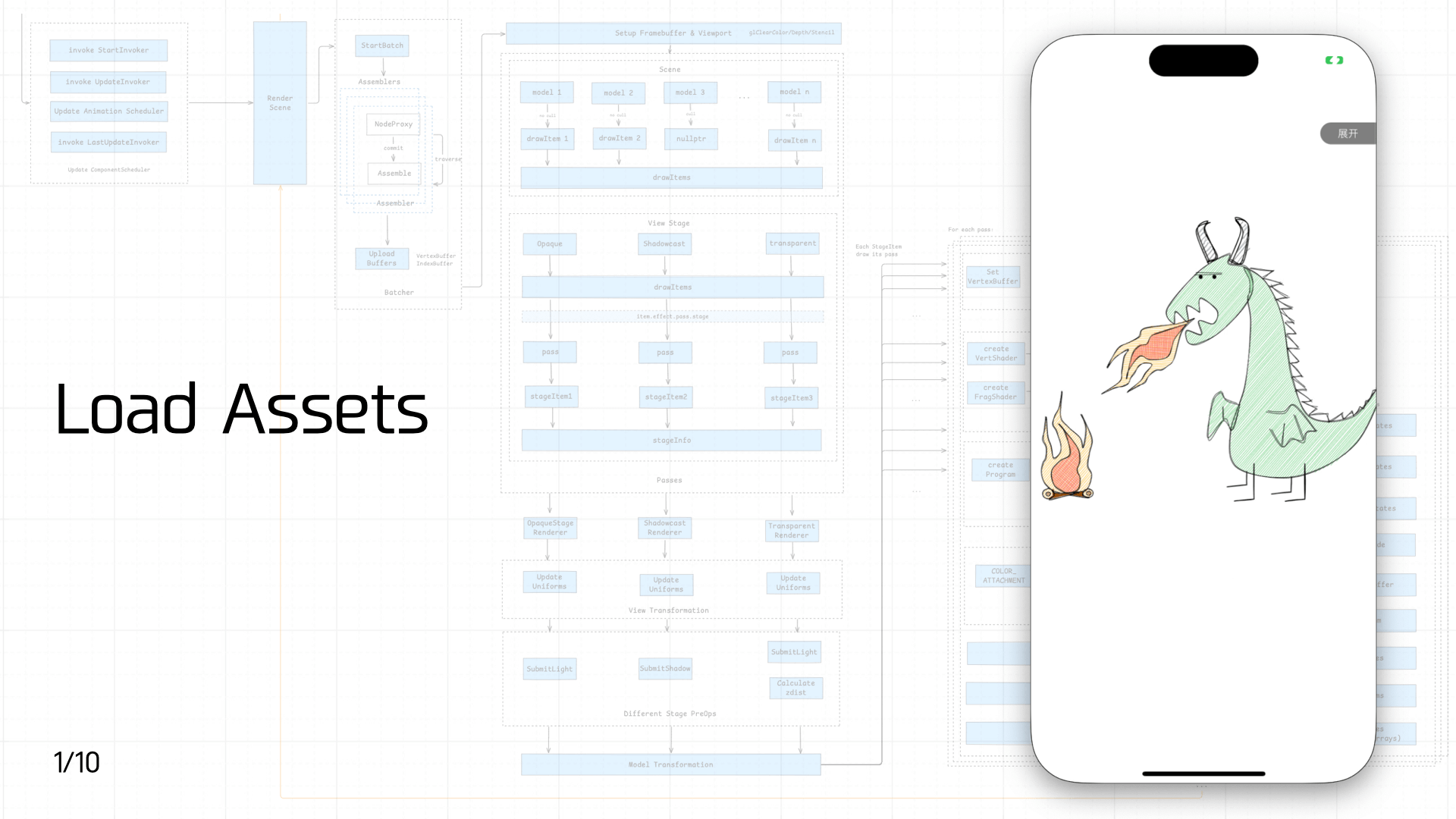 First comes asset loading. As mentioned earlier, game assets split into static assets and script assets. Since static asset loading involves a lot of complexity, this section covers only script asset loading.
There are three types of script assets:
- Built-in scripts: Loaded when the engine starts. These include registering JS Bindings, implementing the
windowobject (basic BOM and Canvas DOM objects), and polyfilling ES standard compliance. The scripts are bundled in the container and loaded immediately when the JS engine launches. This step can support multiple instances and pre-execution to speed up startup. - Entry scripts: The container needs an entry script — similar to HTML on the web — to import the game’s entry assets.
- Dynamically loaded scripts: Imported by the entry assets: game framework code, JS assets from the game bundle, etc.
On the container side, optimizations include offline assets, preload, prefetch, and pre-execution. On the JS engine side, Code Cache can be added to avoid repeated compilation overhead.
3.2 Component Scheduler
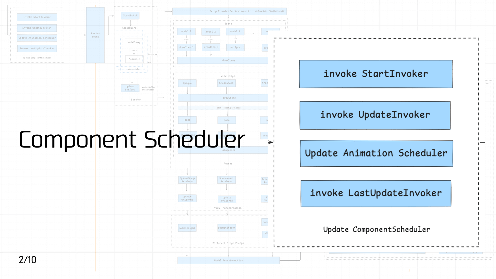 After script assets load and execute, game component code enters the component scheduler for priority scheduling.
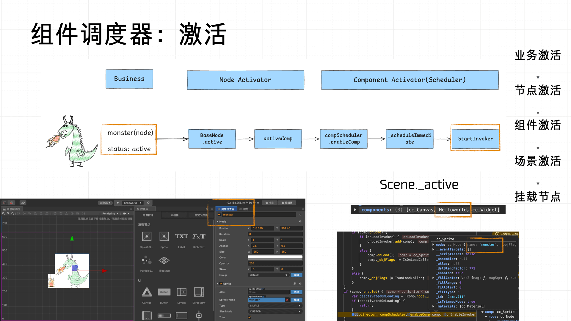
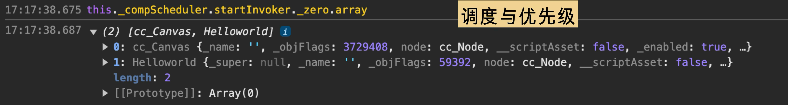
The Cocos component lifecycle is shown on the left in the diagram below. Three key lifecycle phases each have a corresponding scheduler, and each scheduler is designed with three priority queues. Each queue is organized as a linked list, executing registered invokers in order.

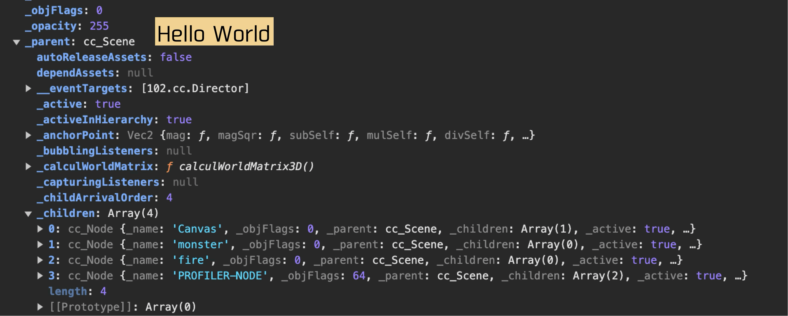
From the business perspective: when a Node is created in the scene editor, developers can name it and toggle the “active” property to set its default activation state. Once a node is marked active, the Load phase hands it off to the Node Activator, which activates the node. The Component Activator (part of the component scheduler) then sequentially activates each component mounted on the node and triggers the activation of the Scene that contains it. Finally, the activated scene attaches the node to the hierarchy tree and registers the component Invokers with the scheduler for unified scheduling and management.
The overall flow:
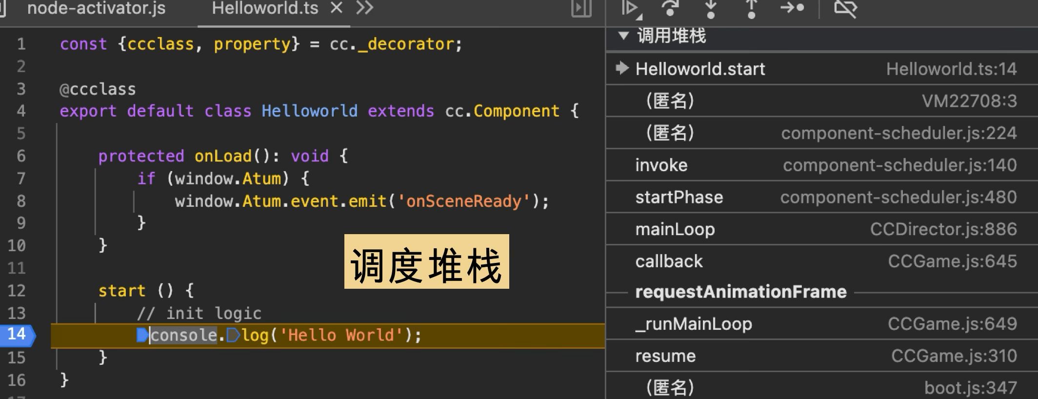
Our demo component logs “Hello World” in the start lifecycle. The call stack looks like this:
3.3 Render Scene
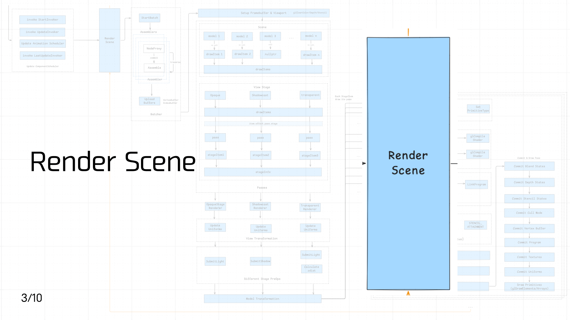 Once the scene is activated and components are mounted, the next step is rendering the scene — which involves calling from JS into Native: Scene data must be passed to the Native side to trigger the Native rendering pipeline.
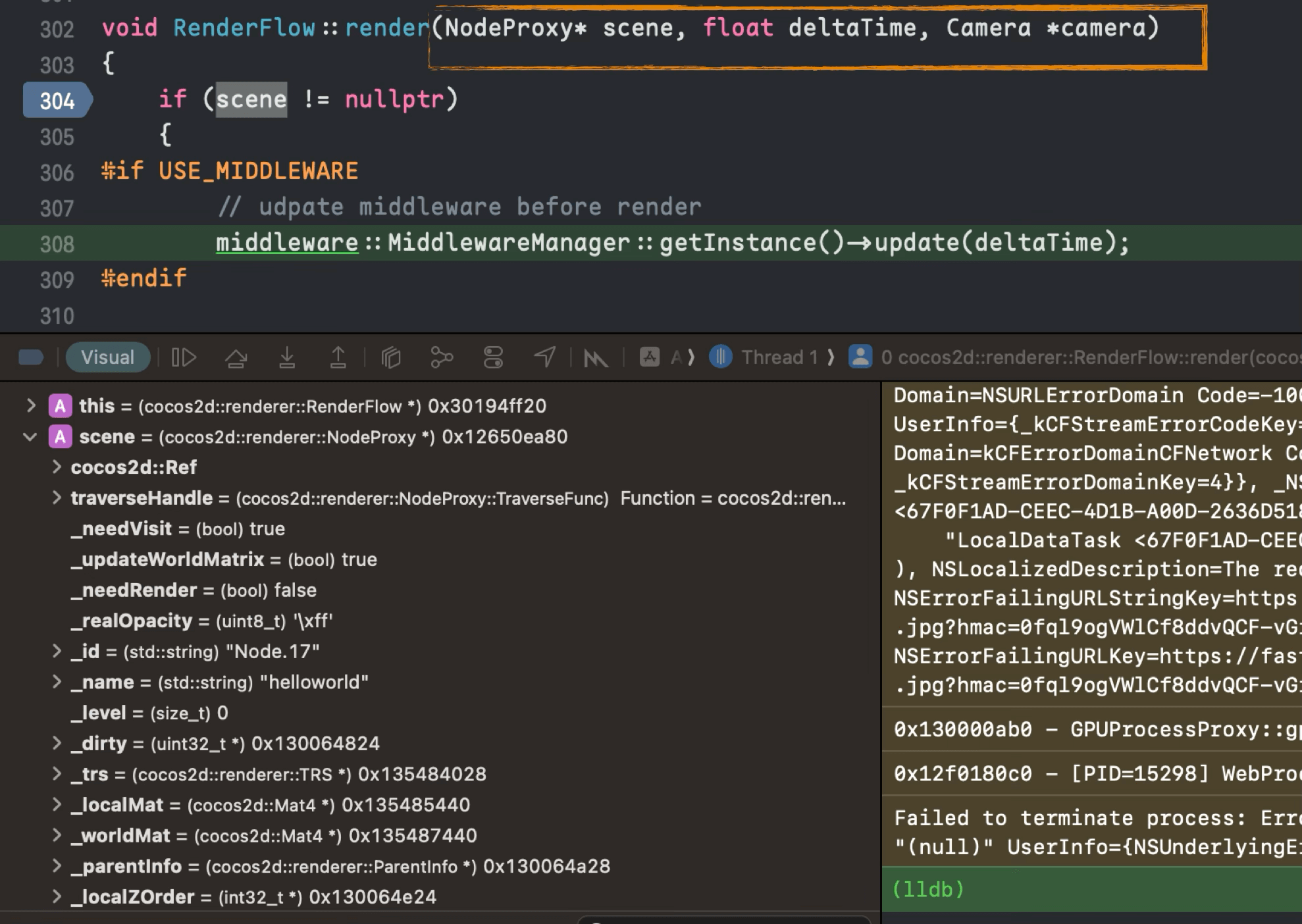
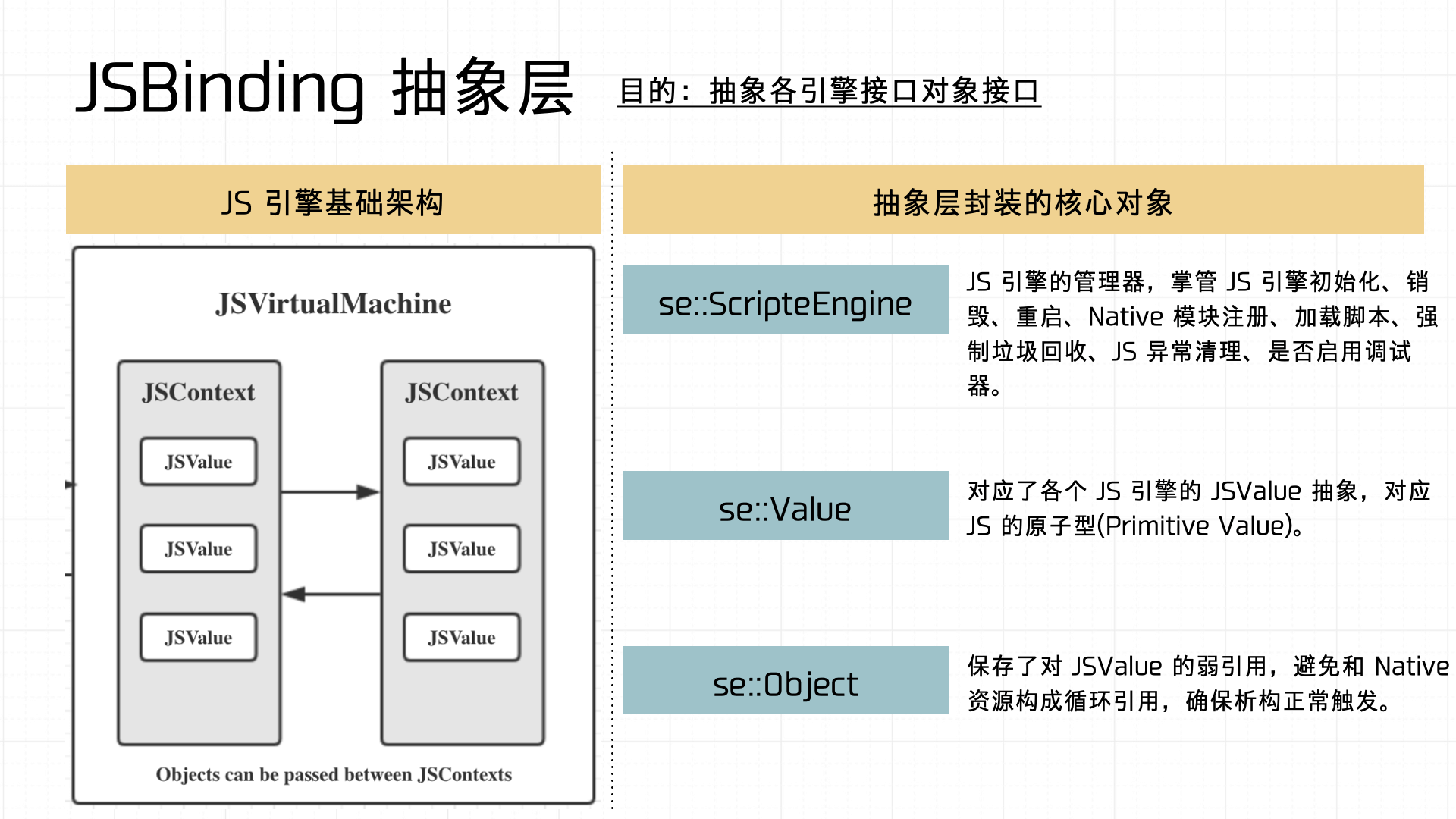
There are many ways for JS and Native to call each other, each suited to different scenarios — we won’t expand on those here. One architectural note worth making: the Binding layer should be abstracted so the container can interface with different JS engine implementations.
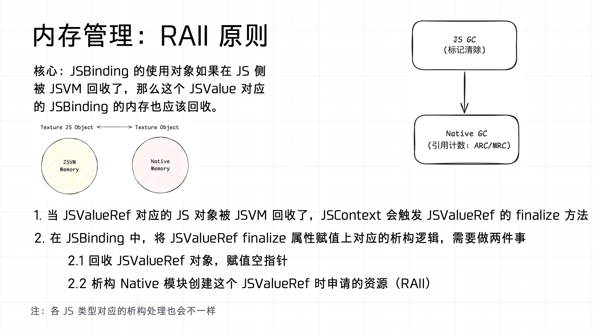
Also important: the Binding must handle GC properly on both sides. Therefore, Binding implementations must follow the RAII principle:
3.4 Batcher
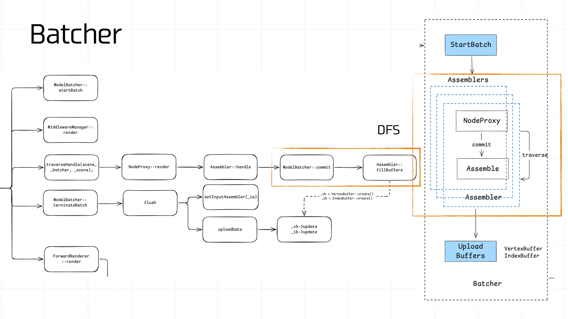
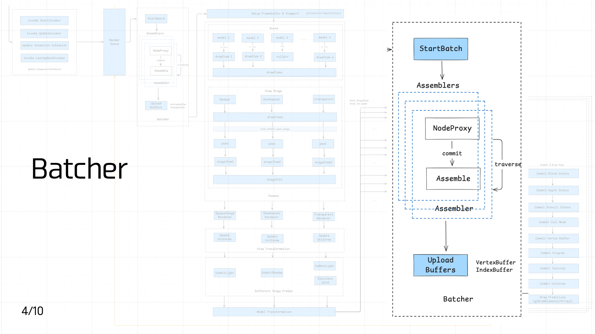 Once Native receives the nodes, they need to be batched. This step is compute-intensive, which is why it’s done on the Native side.
The batching process is complex. The core idea is to traverse the scene’s Nodes via DFS, compute and assemble vertex data (Assembler), and produce a VertexBuffer and IndexBuffer:
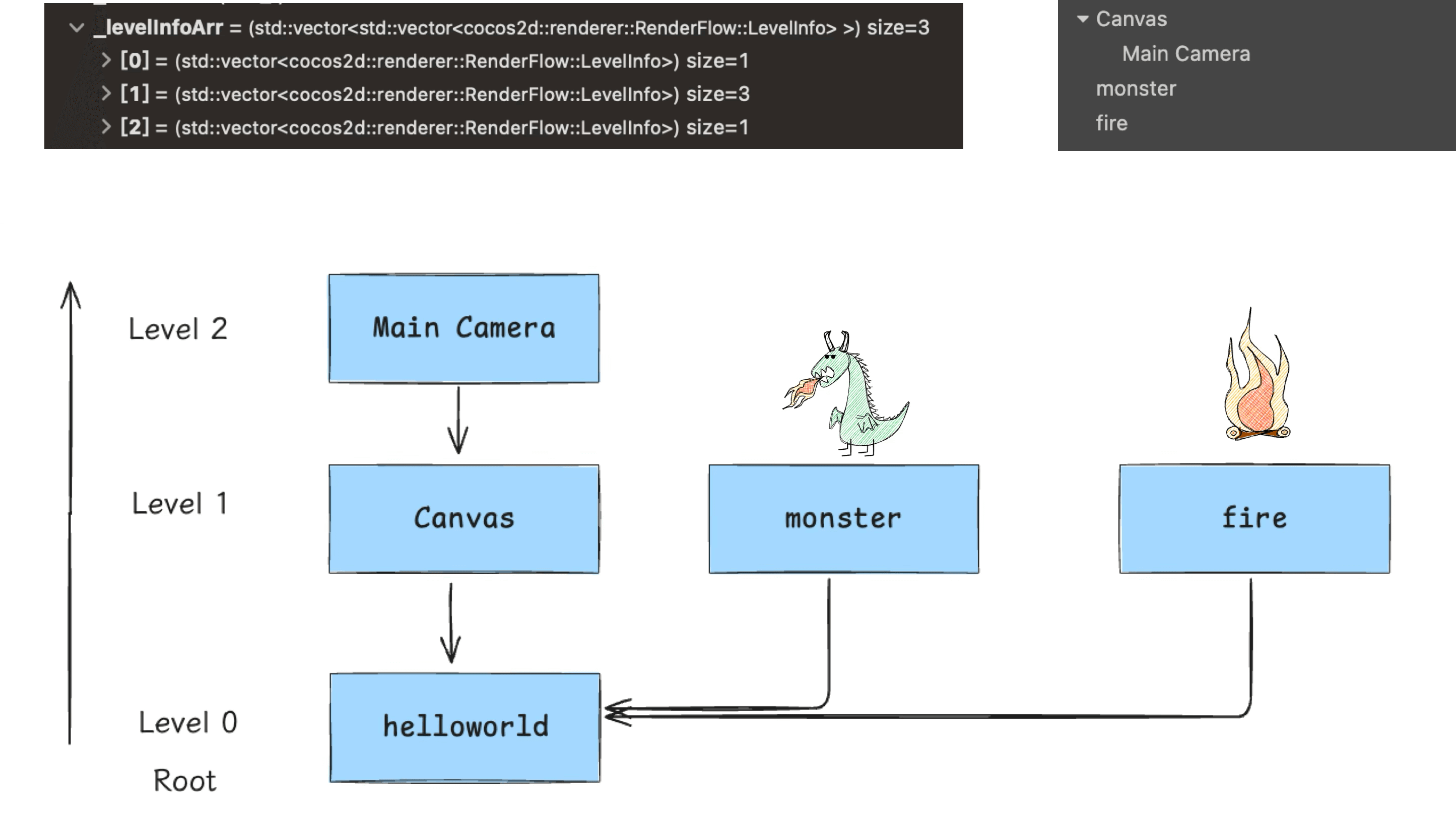
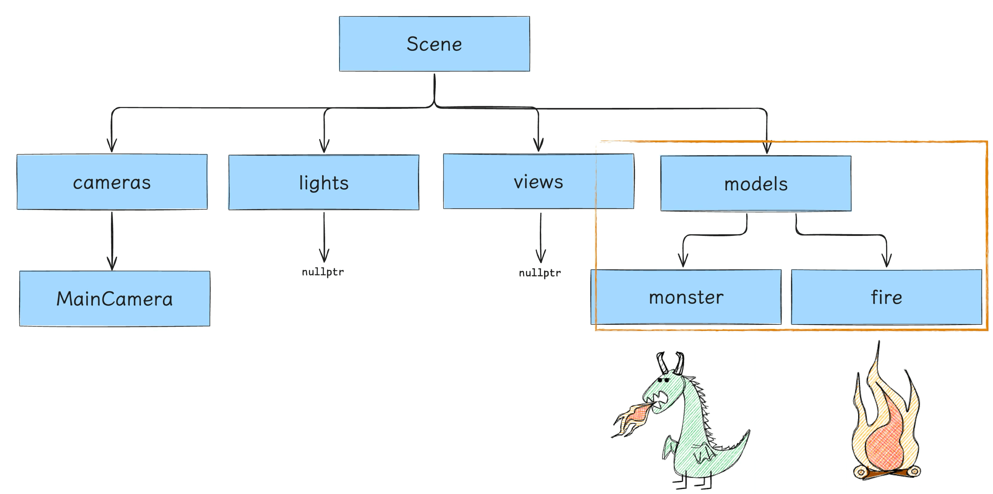
Our demo’s scene tree is relatively simple. Traversal starts from root and goes downward (don’t forget the Camera):
The assembly computation is complex; here I’ll just break down the final result to help readers understand where the data comes from. Our little dinosaur is a Sprite2D — during assembly it’s converted to Texture2D processing. The critical output at this stage is the Mesh Buffer:
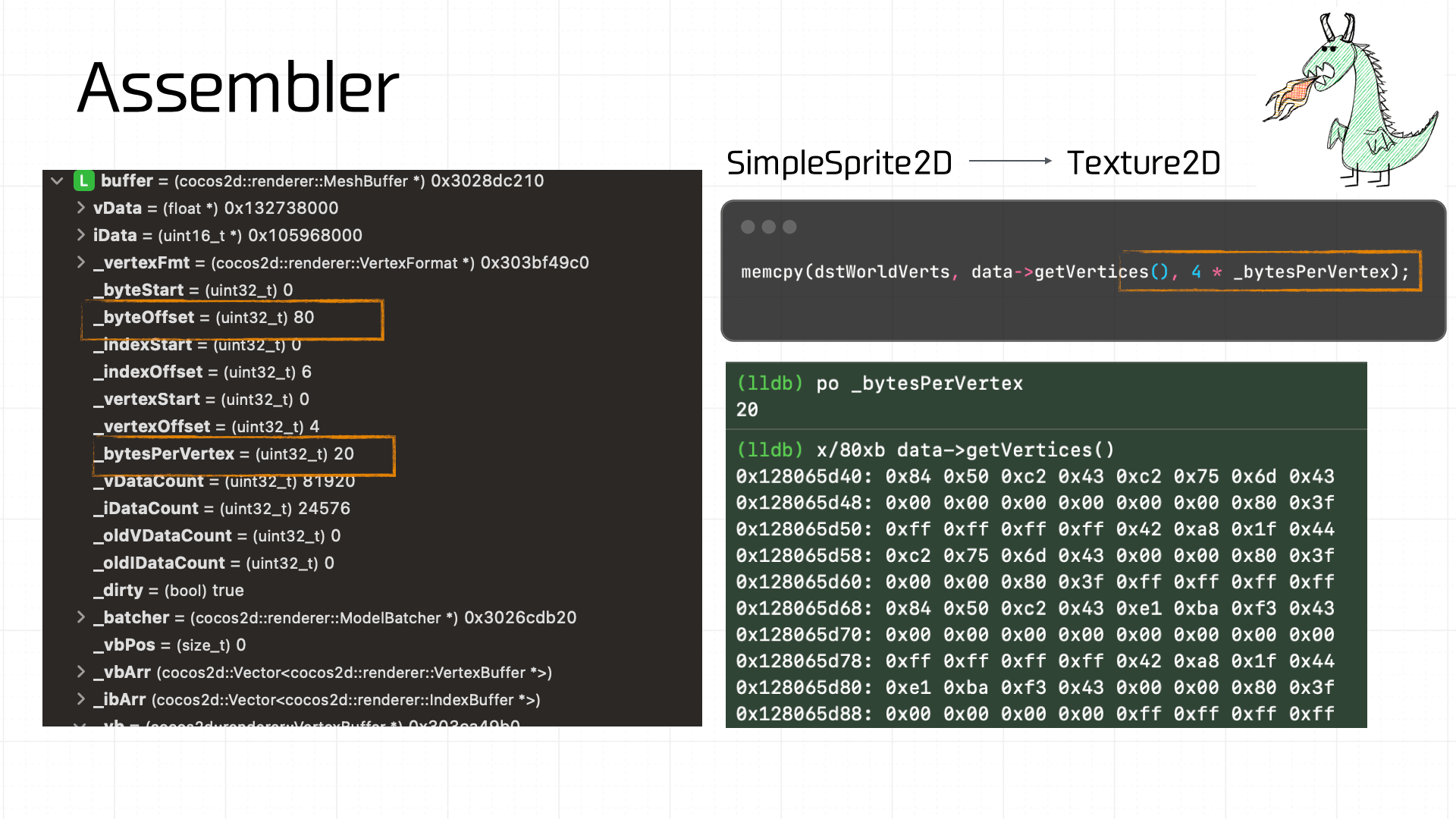
The Mesh Buffer is made up of Vertex Buffers. This assembled Mesh Buffer is 80 bytes total. At 20 bytes per vertex, we can extract 4 Vertex Buffers, and using the a_uv definition and offsets we can recover the UV coordinates for each:
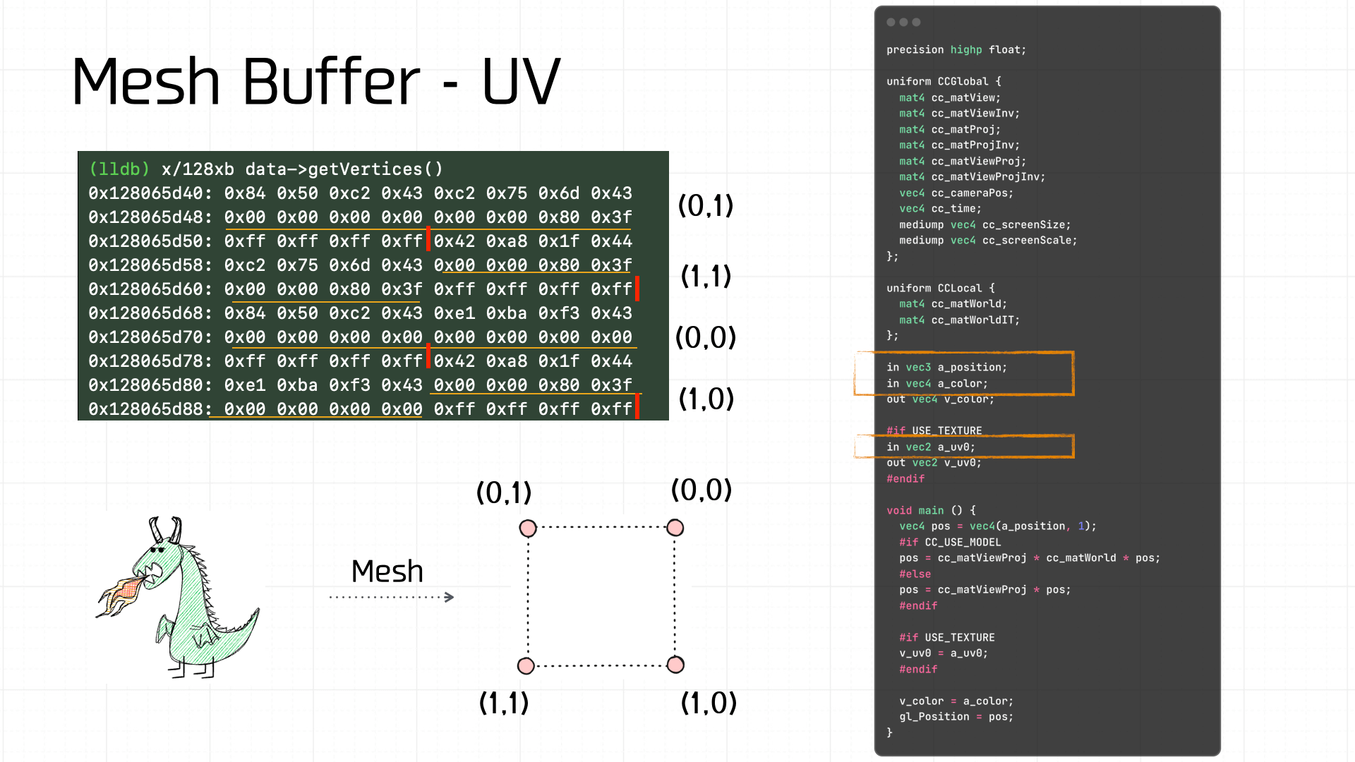
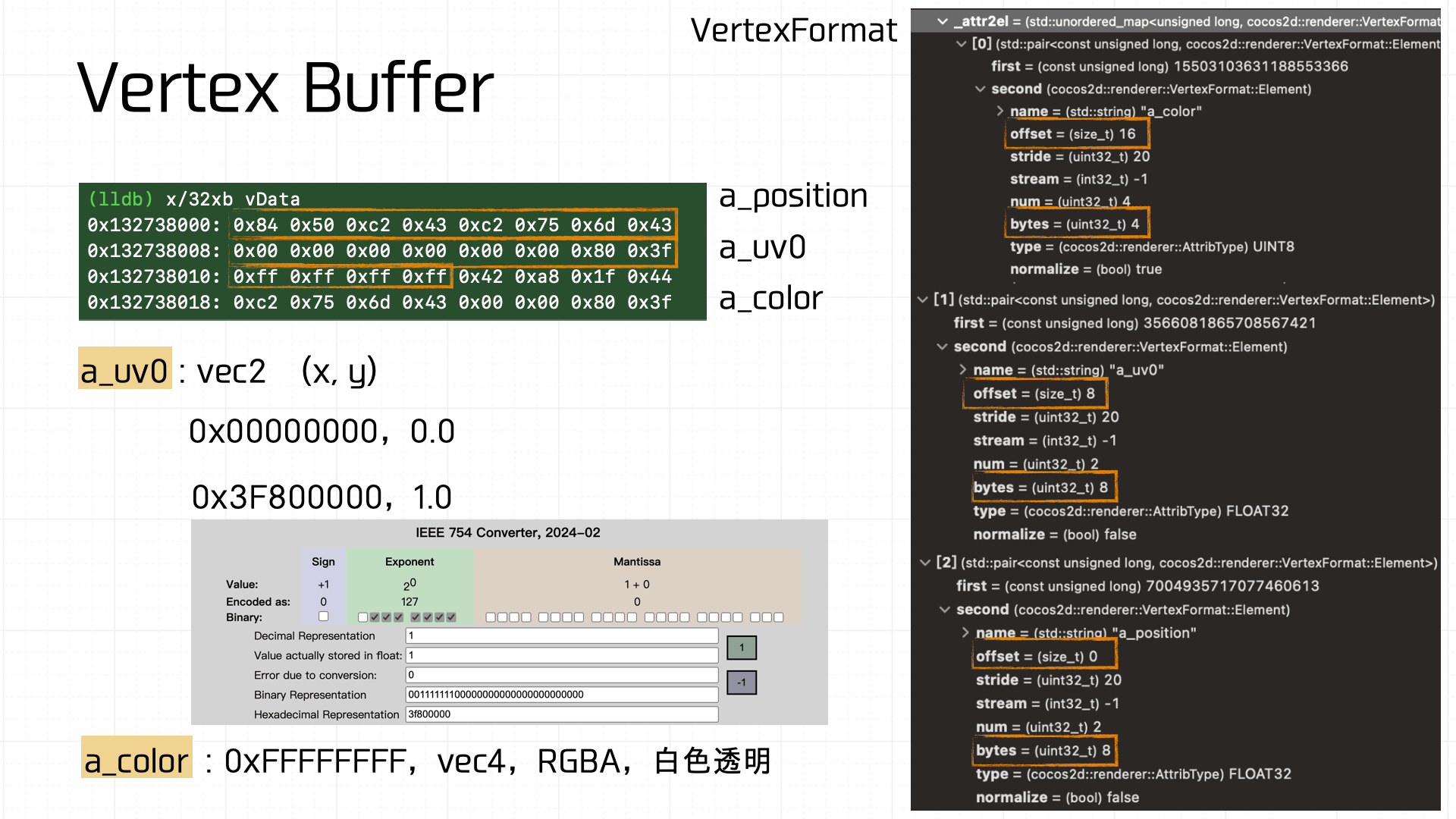
For example, from the vertex shader code we know each Vertex Buffer contains 3 data components:
a_position: offset 0, 8 bytes.vec2— one coordinate.a_uv0: offset 8, 8 bytes.vec2— x, y — evaluates to (0, 1).a_color: offset 16, 4 bytes.vec4— RGBA — value 0xFFFFFFFF, i.e., opaque white.
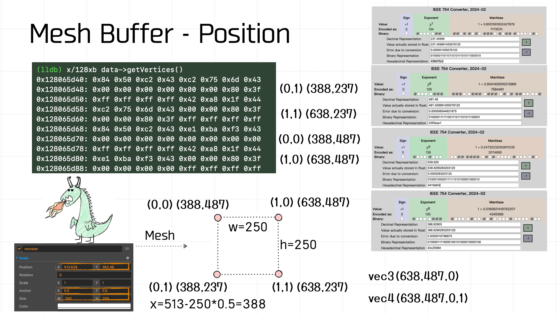
Computing all four vertex coordinates gives us the width, height, and top-left coordinate — and indeed, this data matches exactly what the developer set for the Node’s size and position in the scene editor:
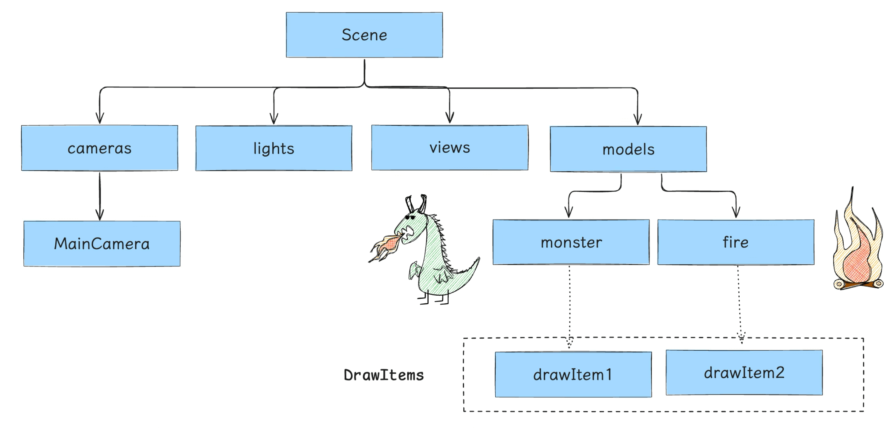
After vertex assembly, the Nodes are placed into the Models list and assembled into models nodes within the Scene Tree:
3.5 Setup
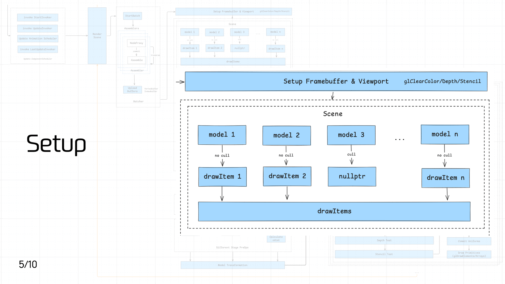 This stage consists of two main operations:
- Setting up the Framebuffer and Viewport
- Converting each Model in the Scene into a DrawItem queue
First, setting up the Framebuffer and Viewport:
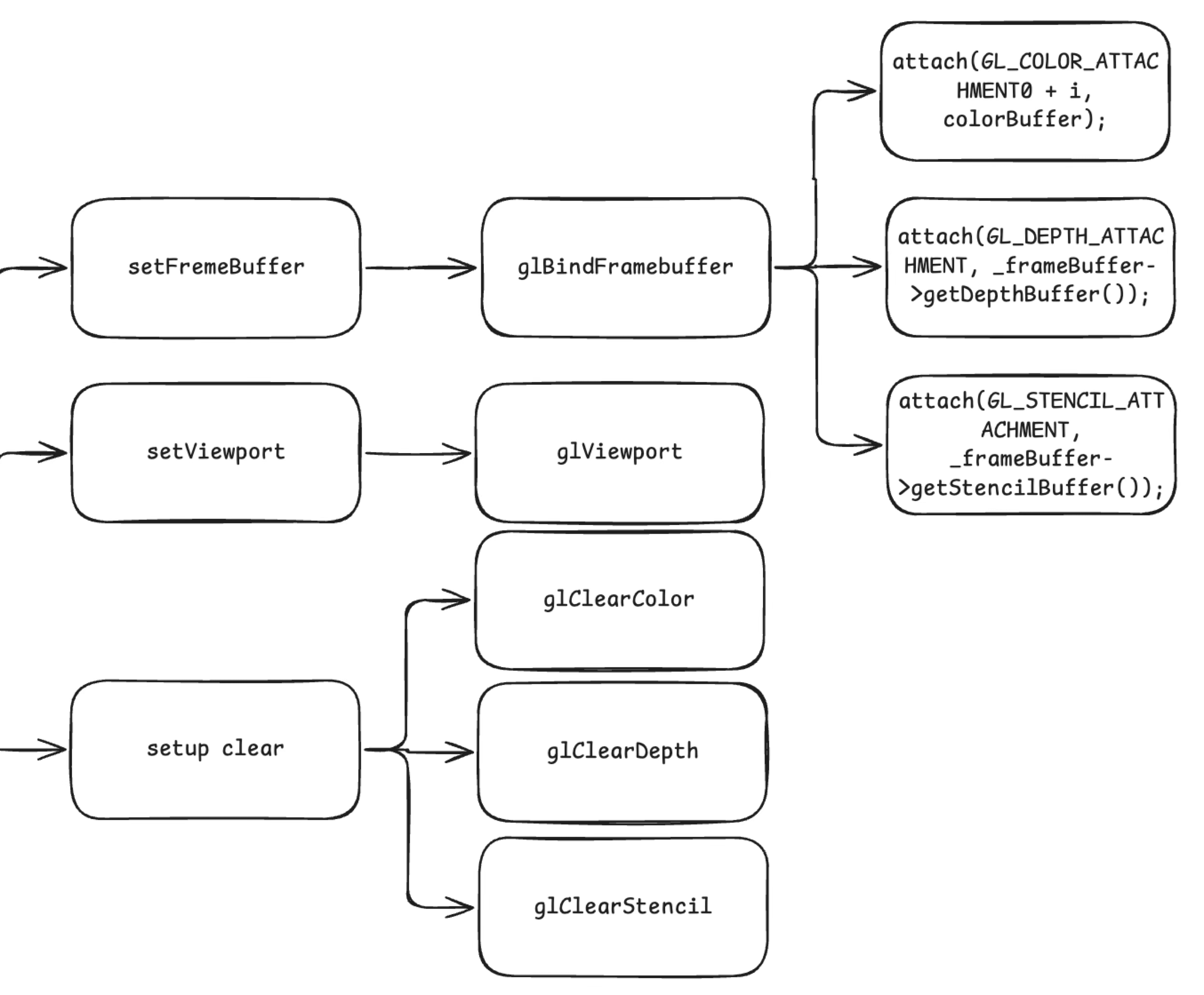
setFrameBuffercallsglBindFramebufferto bind the Framebuffer Object, attaching a color buffer (COLOR_ATTACHMENT, storing rendered color information), a depth buffer (DEPTH_ATTACHMENT, storing per-pixel depth for depth testing), and a stencil buffer (STENCIL_ATTACHMENT, storing stencil test results) — ensuring subsequent drawing has the correct render targets.setViewportcallsglViewportto set the viewport, determining the mapping area of the final render onto the screen.setup clearsequentially callsglClearColor,glClearDepth, andglClearStencilto initialize clear values for the color, depth, and stencil buffers, providing a clean initial state for each frame.
unsigned int fbo; glGenFramebuffers(1, &fbo);
Next, the game engine converts each Model in the Scene into a one-to-one DrawItem. A DrawItem’s data structure:
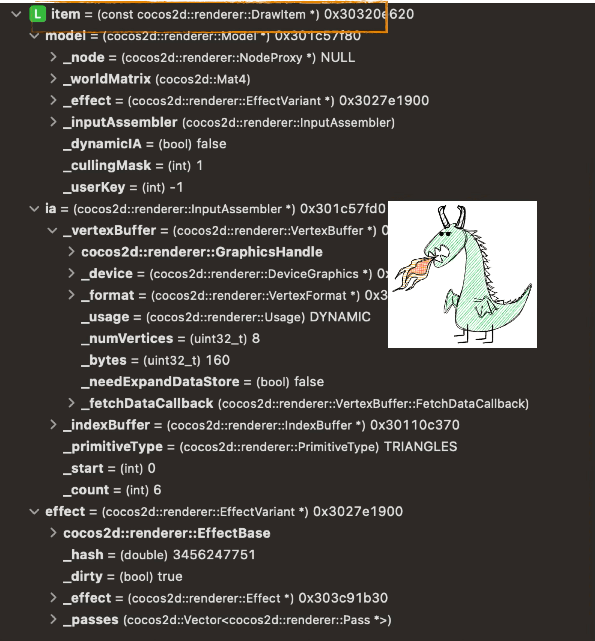
Finally, the engine assembles these DrawItems into a DrawItems queue for subsequent processing:
3.6 Render Stage
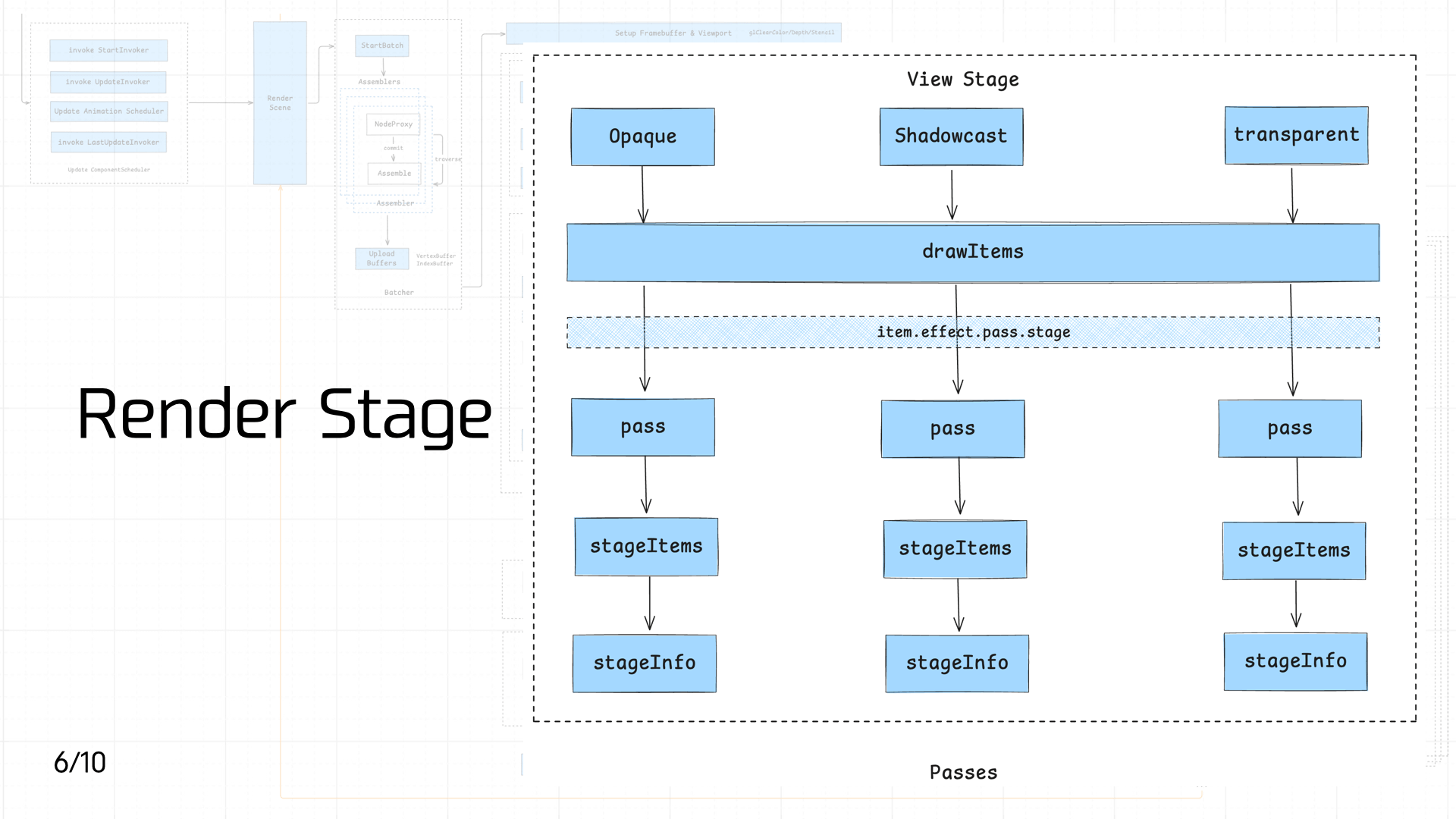 The pipeline enters the Render Stage, where DrawItems are classified and dispatched. Based on each DrawItem’s Material requirements, they’re distributed into three different Passes — Opaque, Shadowcast, and Transparent — corresponding to material properties and shadow casting behavior:
- Opaque: For objects that completely block light, like walls, floors, and character models. Rendered first; uses the depth buffer (Z-Buffer) for occlusion culling, avoiding unnecessary subsequent draws and improving rendering efficiency.
- Shadowcast: Handles shadow casting in the scene. Based on light source information, this pass draws shadows for objects that cast them, adding realism and spatial depth — especially effective in scenes with strong light sources or prominent light/shadow effects.
- Transparent: For semi-transparent objects that allow light through, like glass, water surfaces, and particle effects. Transparent objects typically need depth sorting based on view angle to ensure correct front-to-back layering and avoid visual z-fighting.
By distributing DrawItems into different Passes based on object characteristics, the pipeline can apply effects in a targeted way.
On the business side, you can create a specific Material in code and the pipeline will route it to the corresponding pass:
`// Create a cube mesh const cube = new cc.MeshRenderer(); cube.mesh = cc.GizmoMesh.createBox(1, 1, 1);
// Set material to opaque const opaqueMaterial = cc.Material.create(); opaqueMaterial.initialize({ effectName: ‘builtin-unlit’, technique: ‘opaque’, }); cube.setMaterial(opaqueMaterial, 0); `
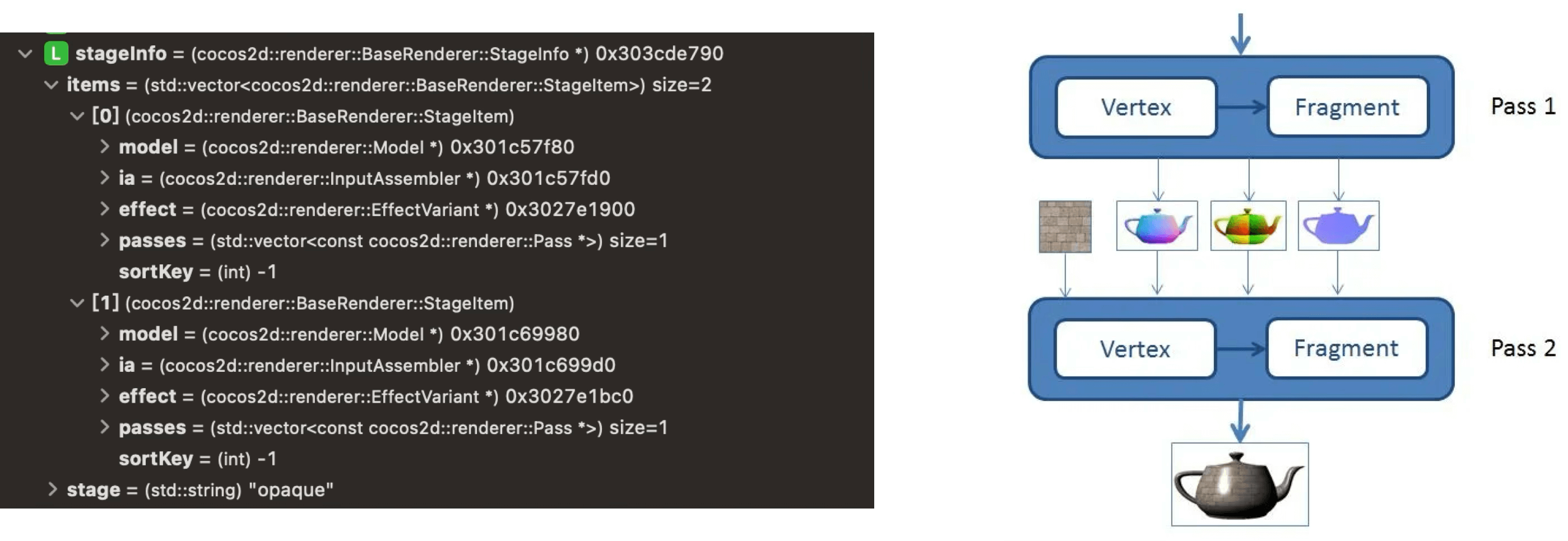
Because our demo is simple, the final StageInfo only includes the Opaque Pass:
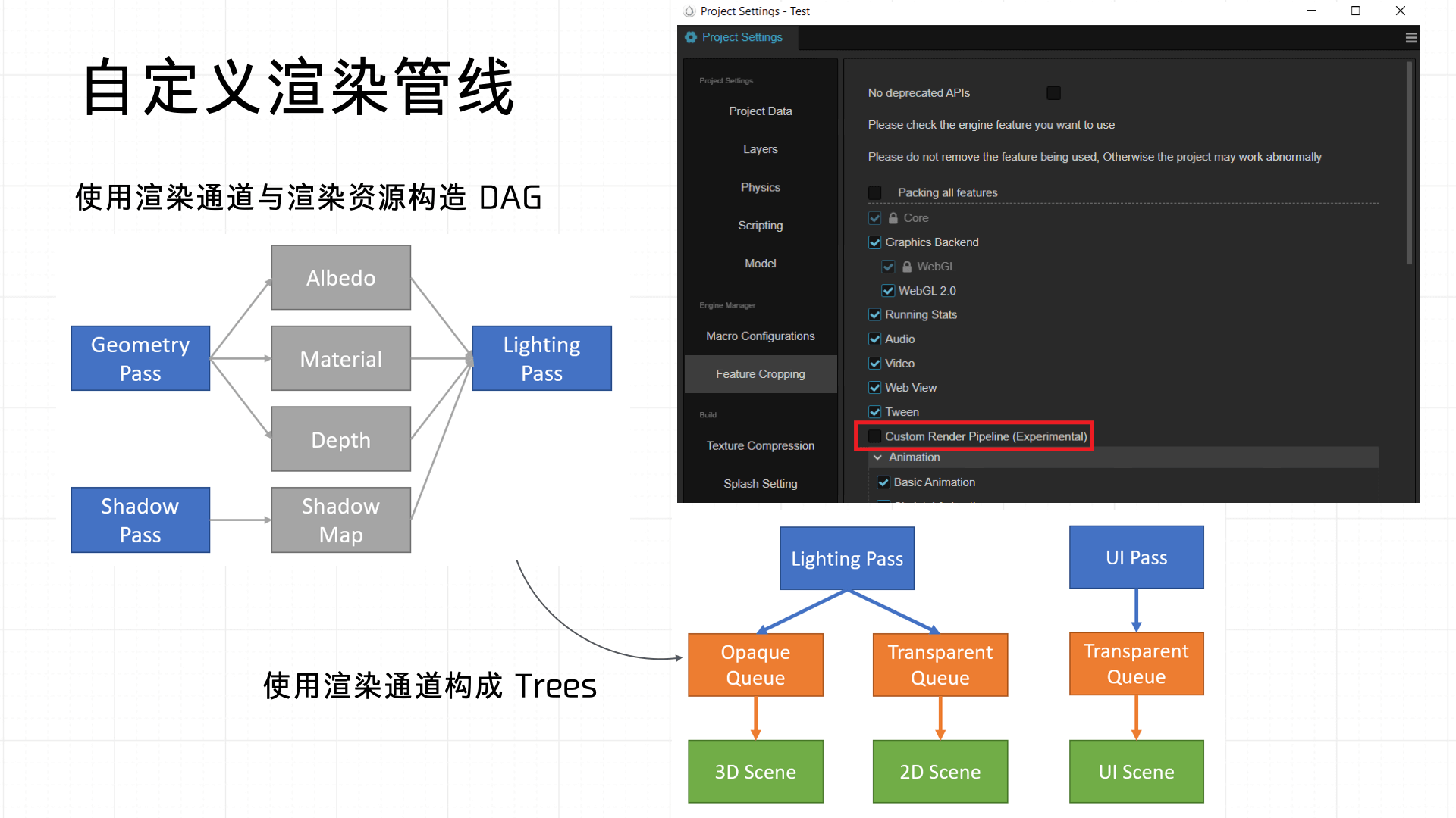
Cocos also supports custom render pipelines — essentially customizing the Passes in this stage. Once defined, they can be applied directly across the Opaque, Shadowcast, and Transparent stages:
3.7 ModelView Transformation
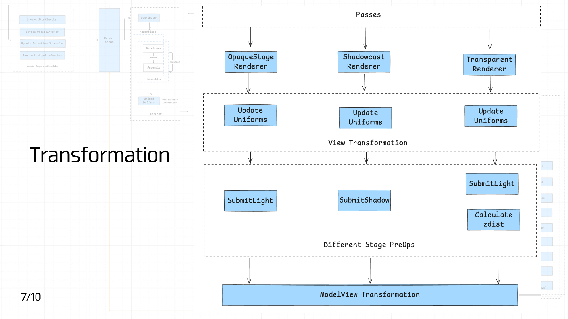 After the Passes, scene DrawItems are sent to the OpaqueStage Renderer, Shadowcast Renderer, and Transparent Renderer based on their properties for initial processing. Each Renderer at this stage primarily updates view-related Uniforms (matrices, material parameters, etc.) to ensure the correct viewpoint and spatial information are available for subsequent rendering. This can be classified as the View Transformation stage — preparing transformation data in view coordinate space.
After that, different render stages apply differentiated pre-processing: opaque and transparent objects both execute SubmitLight to submit lighting information, while the shadow stage exclusively executes SubmitShadow to generate shadow data. Additionally, the transparent stage calculates depth information (Calculate zdist) for depth sorting.
Once all pre-processing completes, everything enters the ModelView Transformation stage, which produces the view-projection matrix and completes the transformation from model space to screen space, enabling subsequent primitive rasterization and pixel shading.
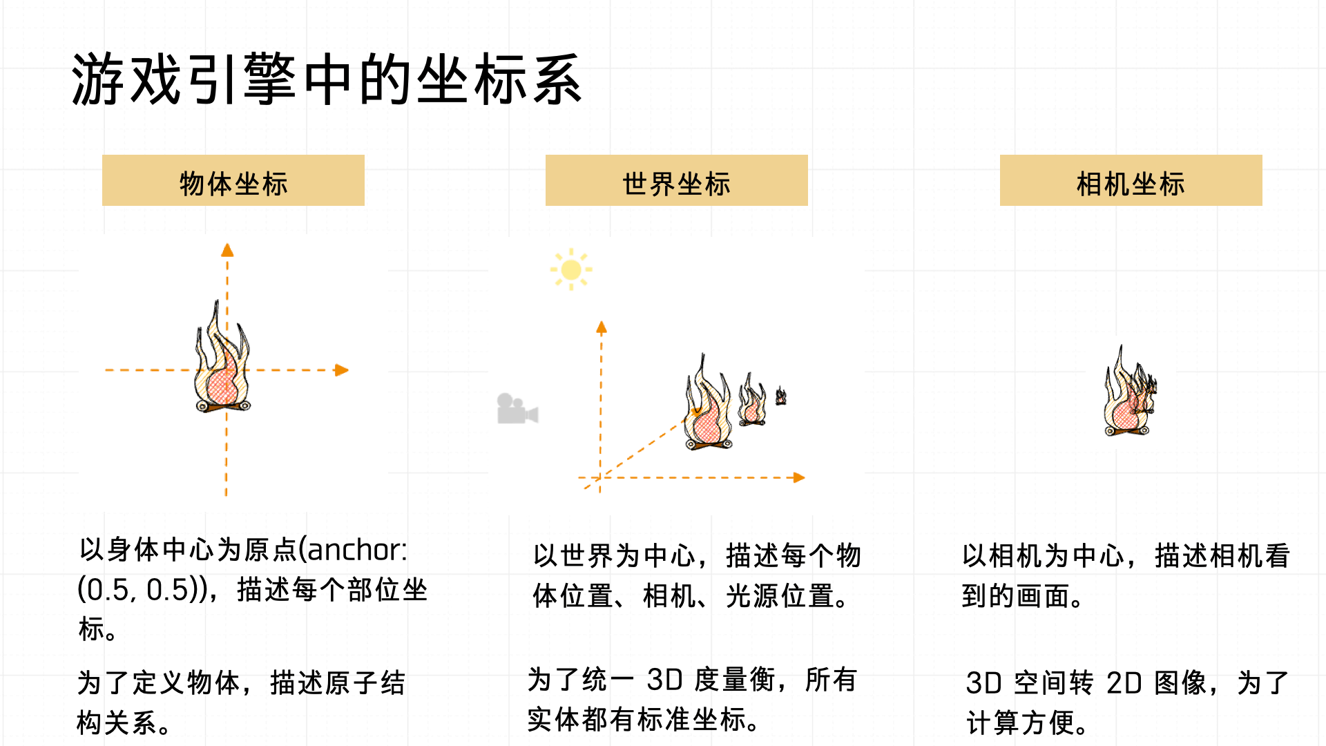
Before diving into ModelView Transformation, let’s define the coordinate systems used in a game:
- Object (local) coordinate system: Origin at the object’s own center (anchor typically set to (0.5, 0.5)). Describes the relative positions of parts within the object — useful for defining the internal atomic structure of complex objects.
- World coordinate system: Origin at the center of the entire scene. Uniformly describes the positions of all objects, cameras, and lights in the scene, ensuring consistent global spatial relationships.
- Camera coordinate system: Origin at the camera’s position. Used to transform 3D space into a 2D image for rendering calculations.
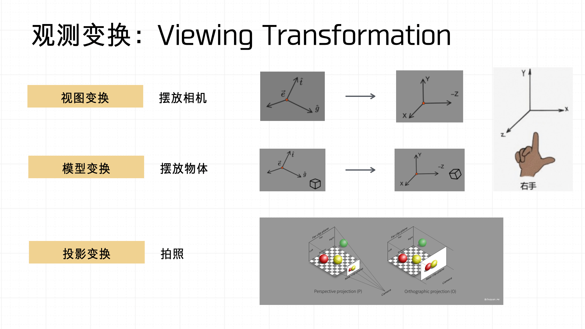
Under this coordinate system, the Viewing Transformation involves three steps: view transformation, model transformation, and projection transformation.
- View transformation: Placing the camera in the scene — defining the camera’s orientation and position.
- Model transformation: Positioning, rotating, and scaling objects in the scene.
- Projection transformation: Like photography — mapping 3D object information onto a 2D screen space through a projection.
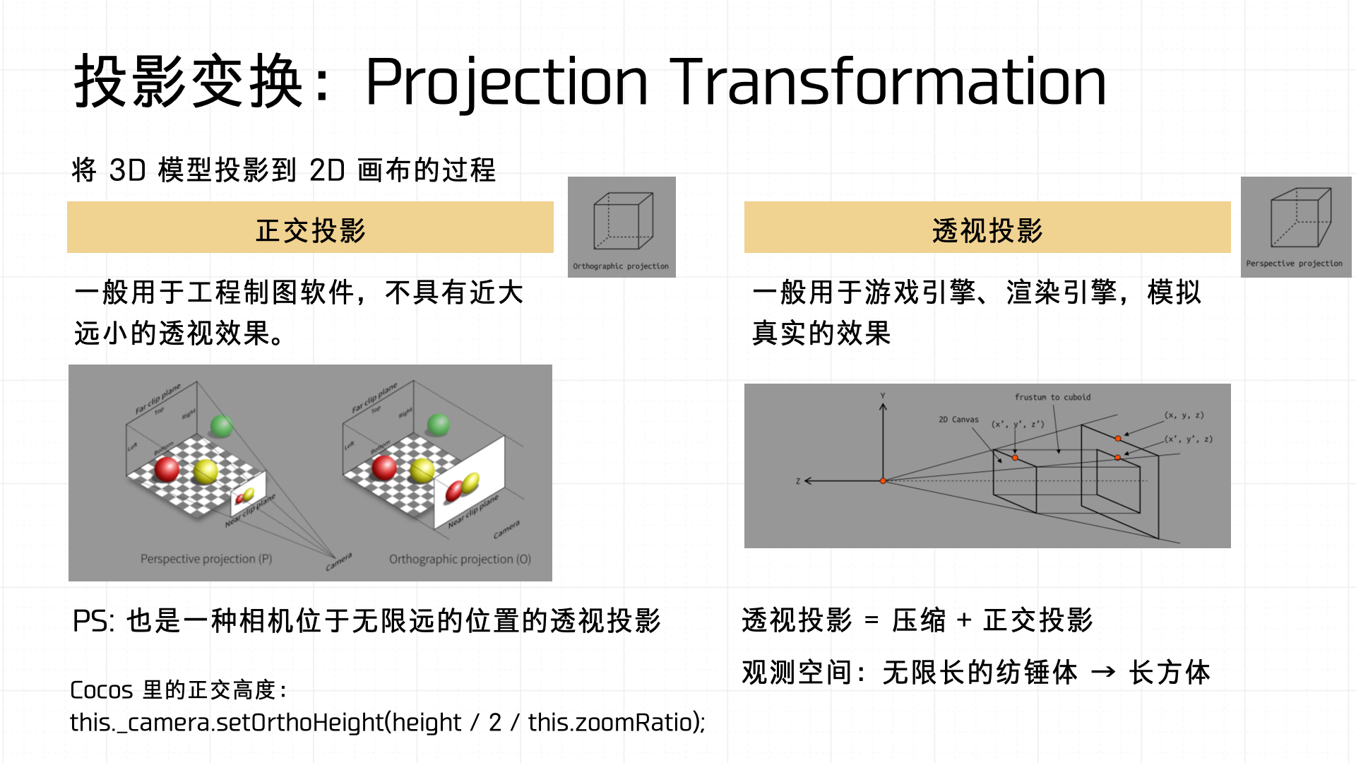
Let’s focus on Projection Transformation, which comes in two forms: Orthographic Projection and Perspective Projection.
- Orthographic projection is common in engineering drawing software — no near-far perspective effect.
- Perspective projection is widely used in games and rendering engines — it more realistically simulates the perspective effect the human eye perceives.
Mathematically, perspective projection is a combination of frustum squishing and orthographic projection — it transforms an infinitely extending view space (frustum) into a convenient box for computation.
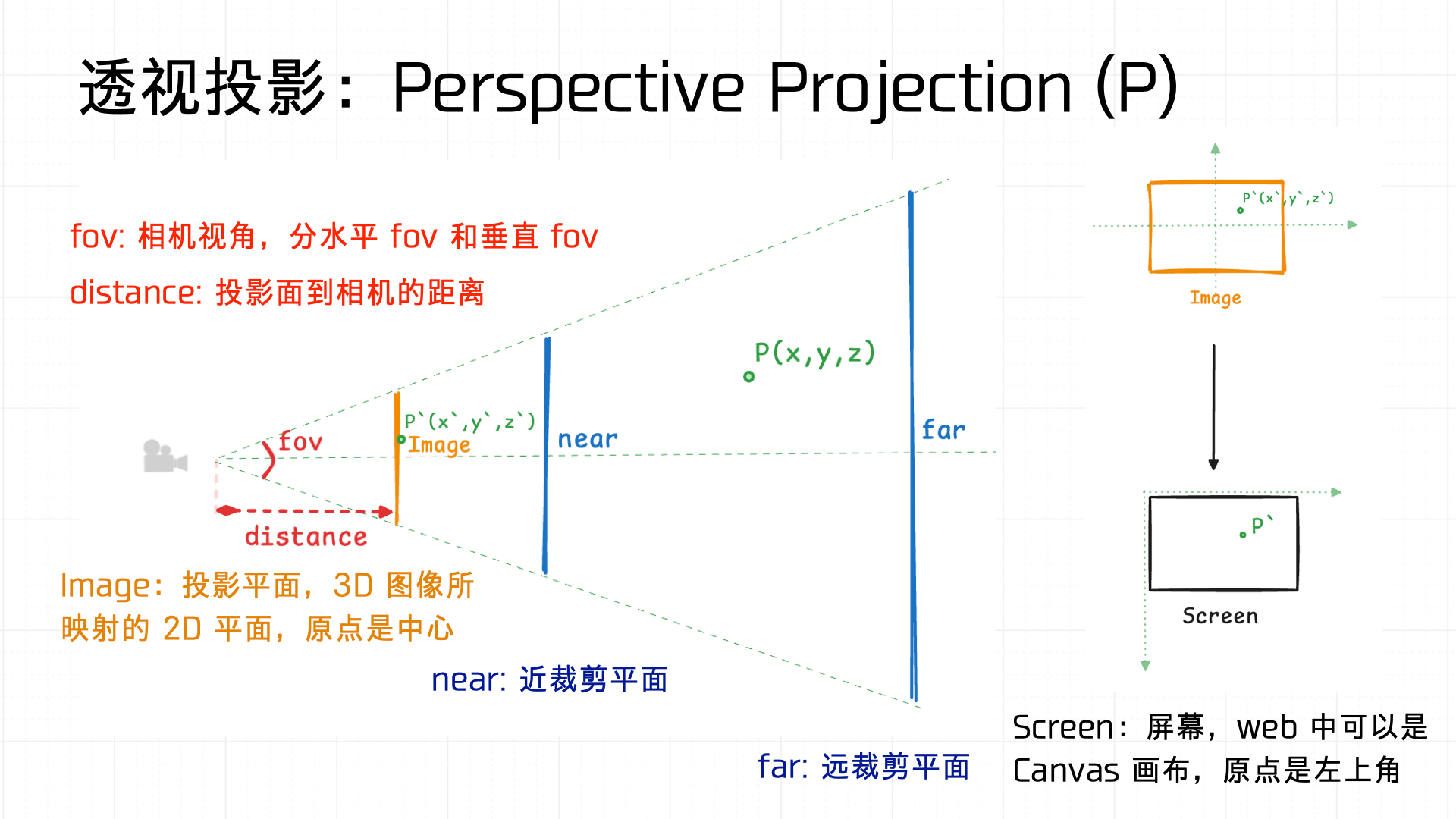
A quick illustration: fov (field of view) defines the camera’s viewing angle width — there’s a horizontal fov and a vertical fov. distance defines the distance from the projection plane to the camera. The view space is defined by near and far clipping planes that bound the rendering range. Using similar triangles, the 3D space is ultimately mapped to a 2D screen (Canvas).
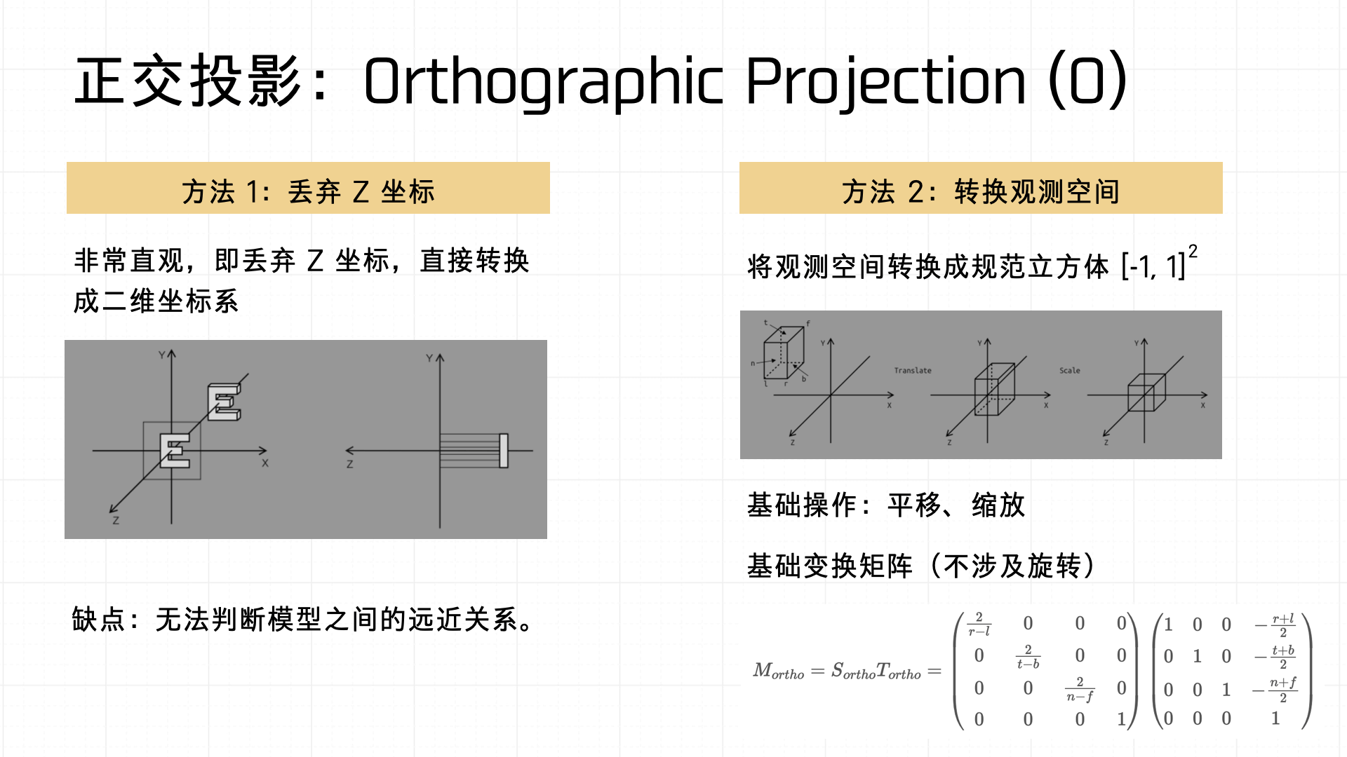
Now for the other type — Orthographic Projection. Two common implementations:
- Simply drop the Z coordinate, converting 3D objects to 2D directly. Intuitive but can’t express spatial depth.
- Transform the view space into a normalized cube, then apply a transformation matrix.
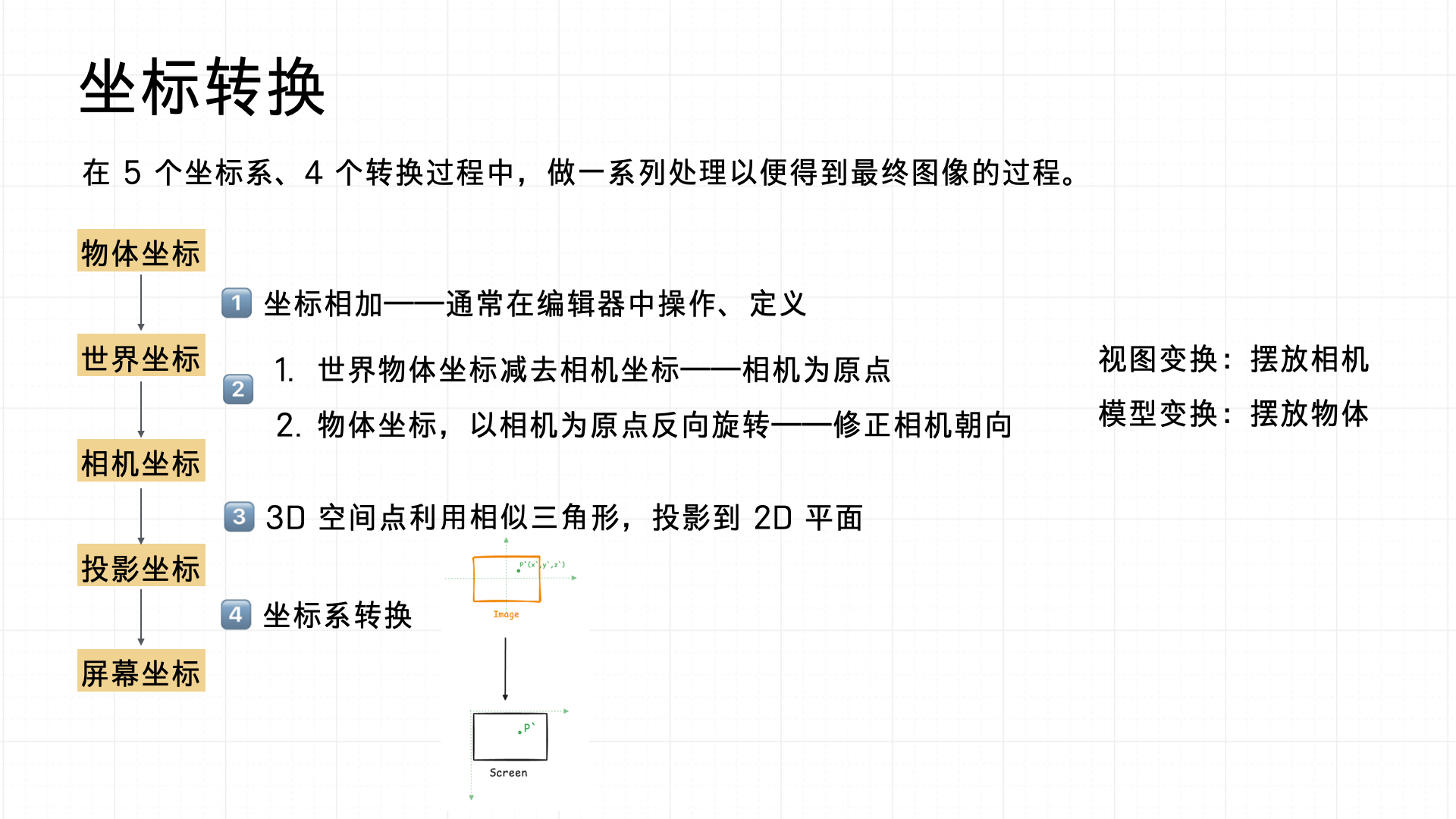
In summary, the coordinate transformation flow is: object coordinates → world coordinates → camera coordinates → projected coordinates → screen coordinates.
- In the editor, define coordinate relationships to place objects in the scene.
- Apply view transformation to position the camera, and model transformation to position objects.
- Apply projection transformation to project 3D space onto 2D.
- Finally, convert to screen coordinates for correct on-screen rendering.
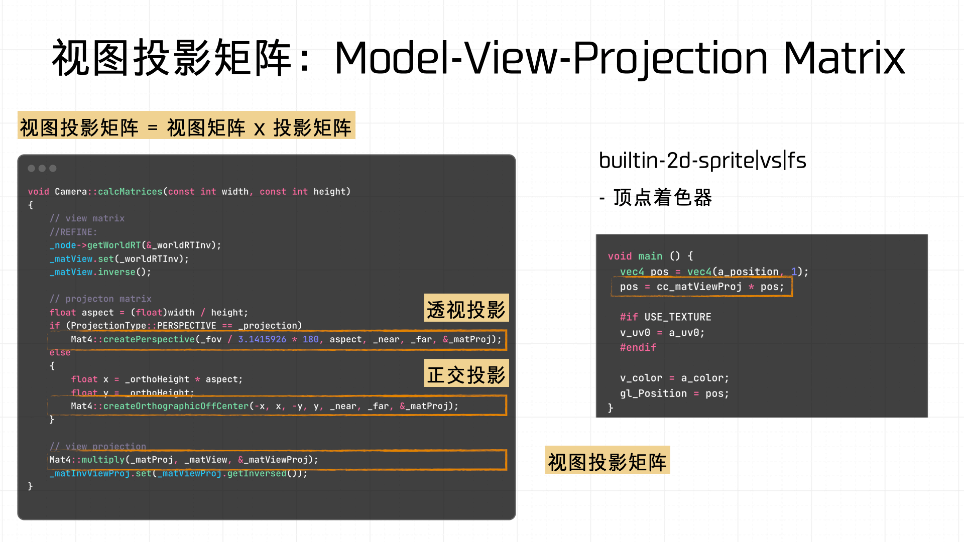
This process produces the View Matrix and Projection Matrix; multiplying them gives the Model-View-Projection (MVP) Matrix. Let’s look at how each is computed using our demo’s breakpoint data.
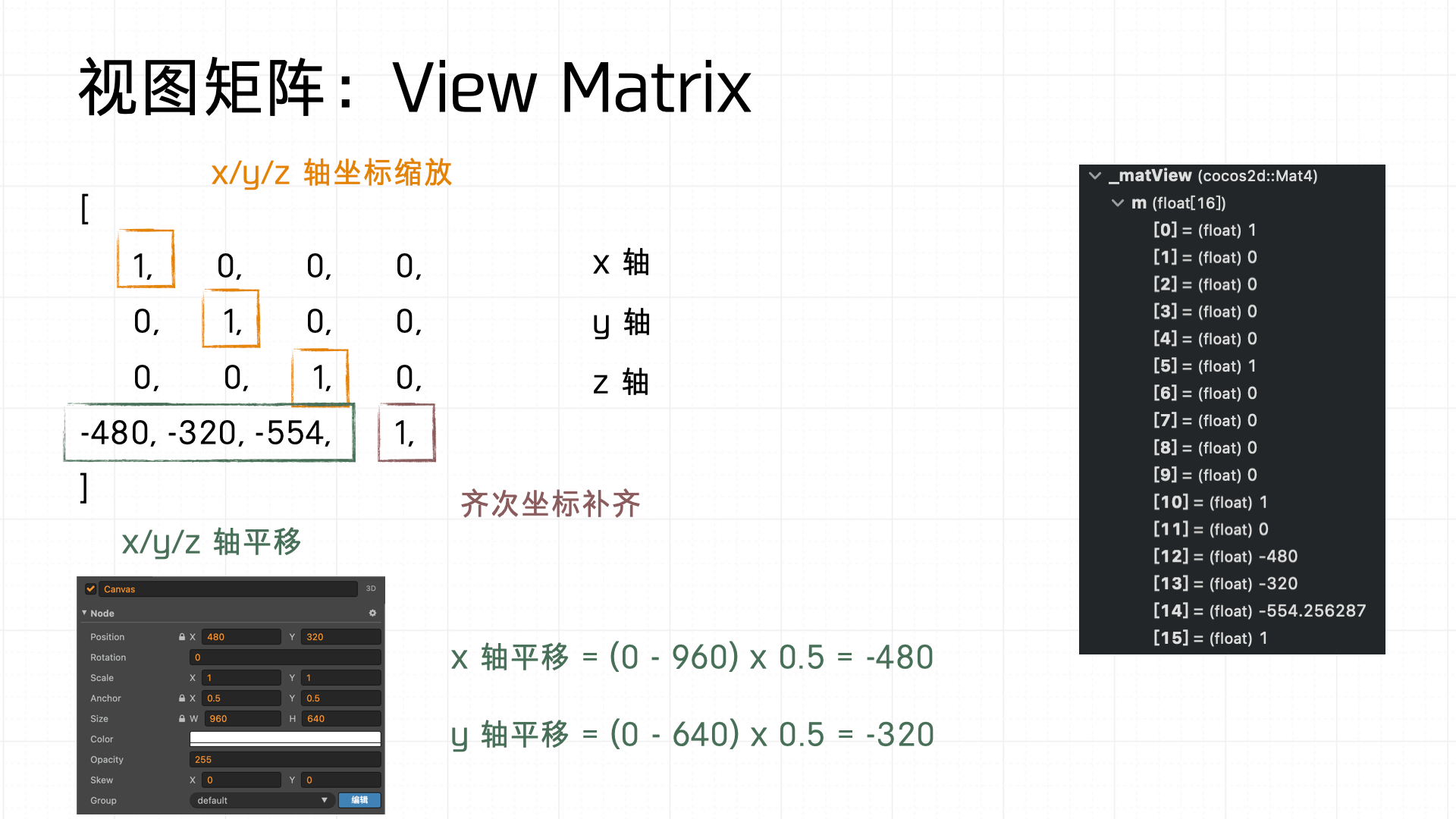
First, the View Matrix — it transforms world coordinates to camera coordinates, including axis scaling and translation. In practice this involves homogeneous coordinate padding to ensure valid matrix operations.
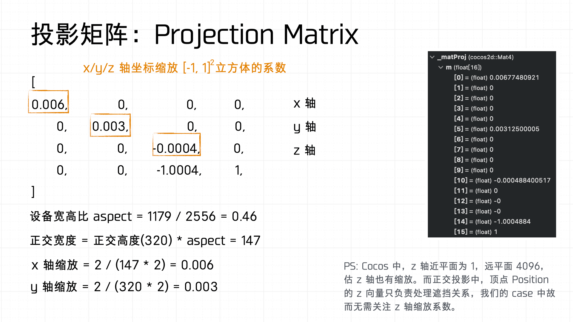
Next, the Projection Matrix — maps camera space to Normalized Device Coordinates (NDC). The scaling coefficients in the matrix are computed from the screen’s aspect ratio and the configured orthographic height.
The final rendering step uses the MVP Matrix (Model-View-Projection Matrix) — a combination of the view and projection matrices, used for final vertex transformation and shader rendering calculations.
3.8 Link Program
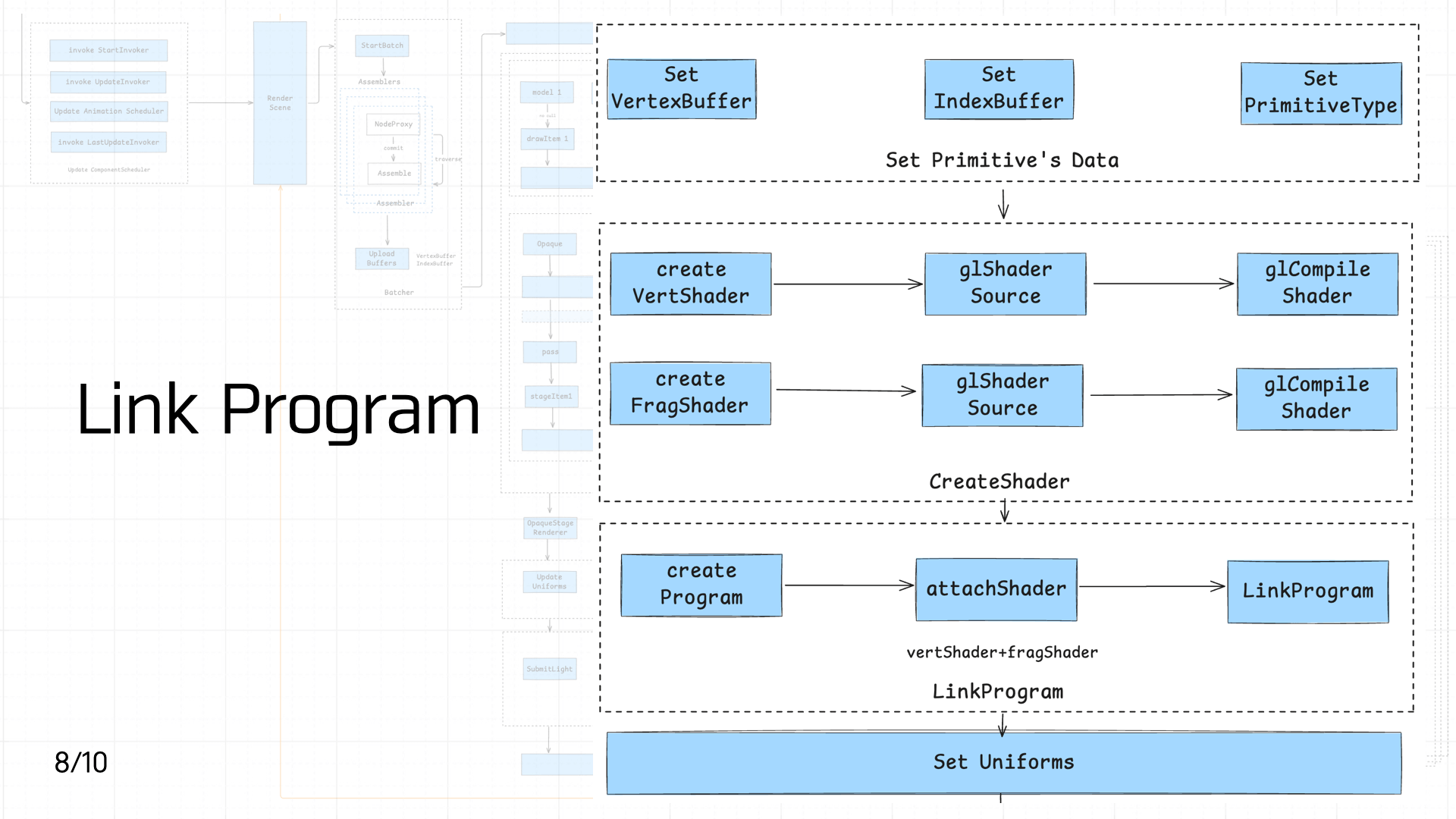 Next comes shader creation and linking. First, creating the primitive:
Then creating the vertex shader and fragment shader:
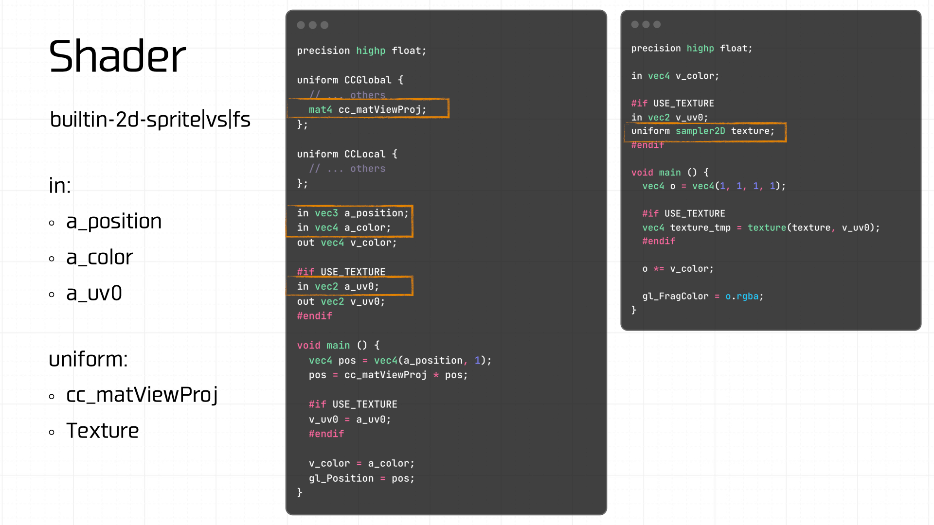
Worth noting: Cocos has 11 built-in shaders. The first 5 handle 2D rendering, builtin-clear-stencil|vs|fs clears the stencil buffer, shaders 7–10 handle 3D rendering, and the last handles 3D lighting:
- builtin-2d-spine|vs|fs
- builtin-2d-graphics|vs|fs
- builtin-2d-label|vs|fs
- builtin-2d-sprite|vs|fs
- builtin-2d-gray-sprite|vs|fs
- builtin-clear-stencil|vs|fs
- builtin-3d-trail|particle-trail:vs_main|tinted-fs:add
- builtin-3d-trail|particle-trail:vs_main|tinted-fs:multiply
- builtin-3d-trail|particle-trail:vs_main|no-tint-fs:addSmooth
- builtin-3d-trail|particle-trail:vs_main|no-tint-fs:premultiplied
- builtin-unlit|unlit-vs|unlit-fs
The demo uses a built-in shader template.
Next, create the shader program and link the vertex and fragment shaders to it. Then set the required Uniform variables — including the texture and the view-projection matrix computed in the previous step:
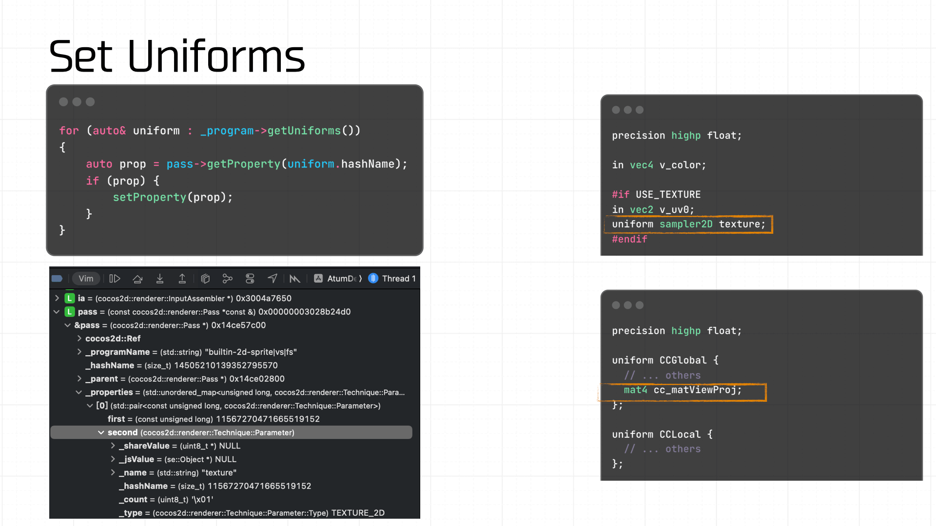
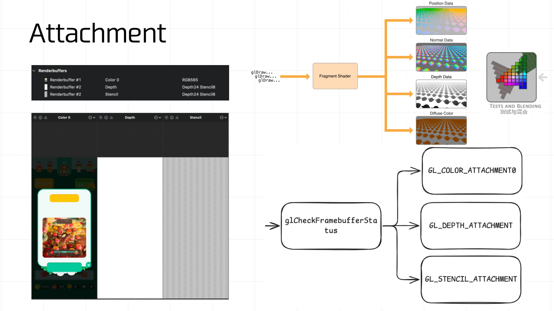
At this point, the Framebuffer will have the color attachment, depth attachment, and stencil attachment:
Note that a freshly created Framebuffer cannot be used immediately — it isn’t yet complete. A complete Framebuffer requires:
- At least one attached buffer (color, depth, or stencil).
- At least one
GL_COLOR_ATTACHMENT. - All attachments must be complete (memory allocated).
- If Multisampling is enabled, all buffers must have the same sample count.
Therefore, use glCheckFramebufferStatus to verify completeness:
GLenum status = glCheckFramebufferStatus(GL_FRAMEBUFFER); if (status != GL_FRAMEBUFFER_COMPLETE) { // ... // notify native: getInstance()->glErrorCallback(GL_ERROR, errMsg); return; }
3.9 Blend & Test
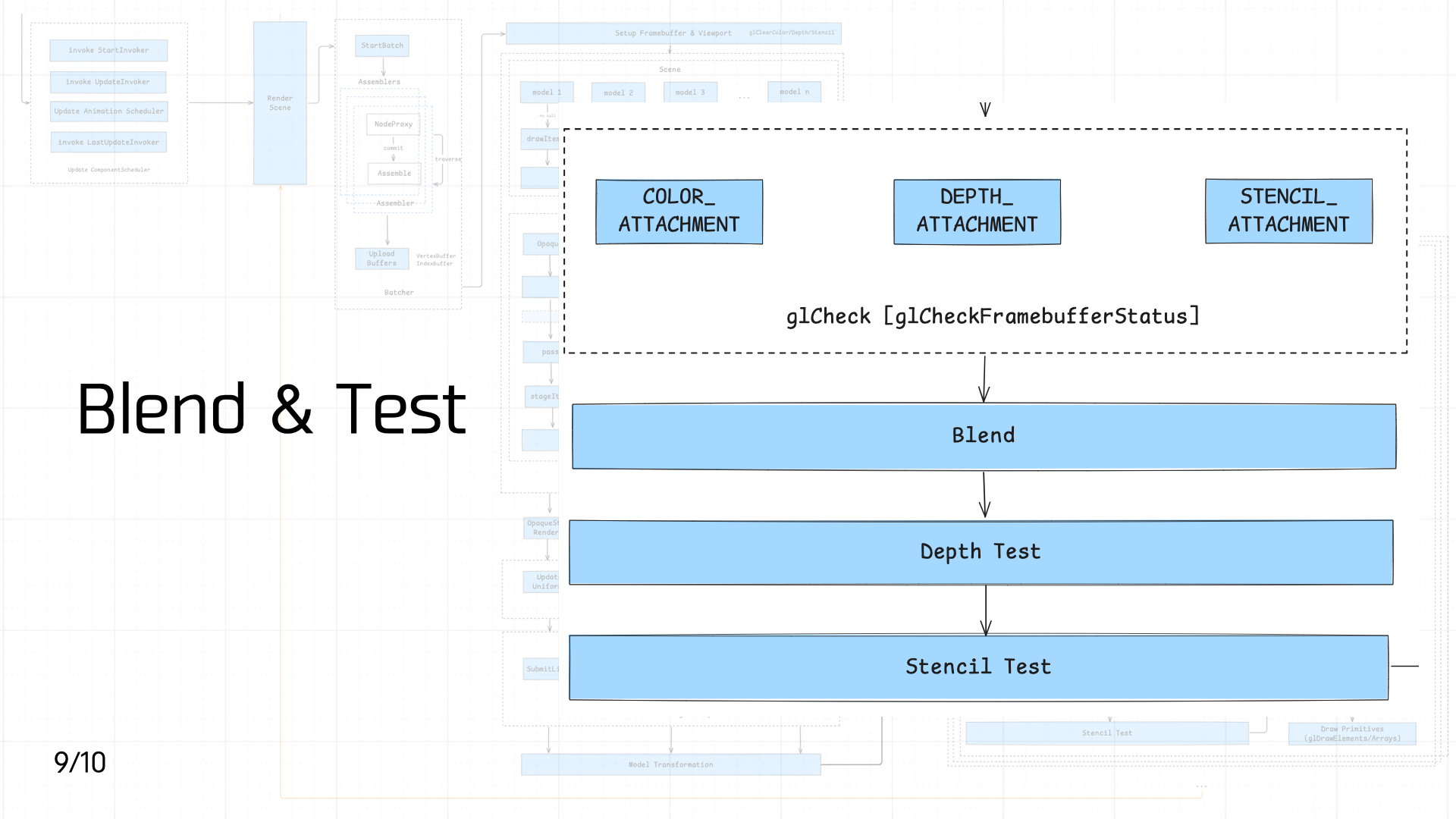 Next comes Blend, Depth Test, and Stencil Test in sequence.
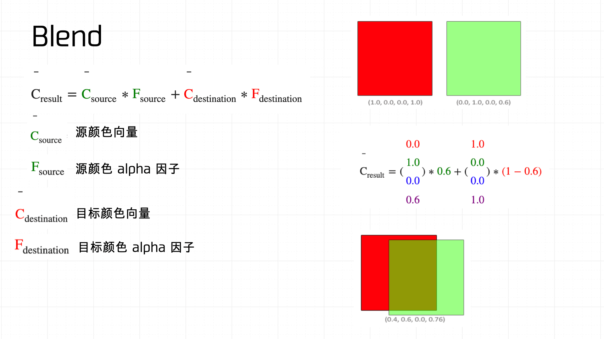
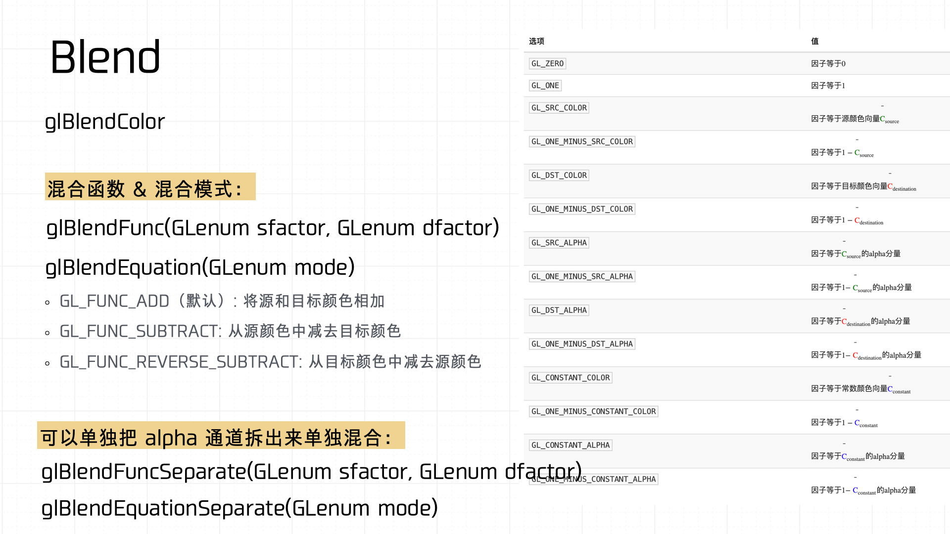
First, Blend — literally blending two colors together. The diagram below shows how the blend equation works:
Common blend functions in OpenGL:
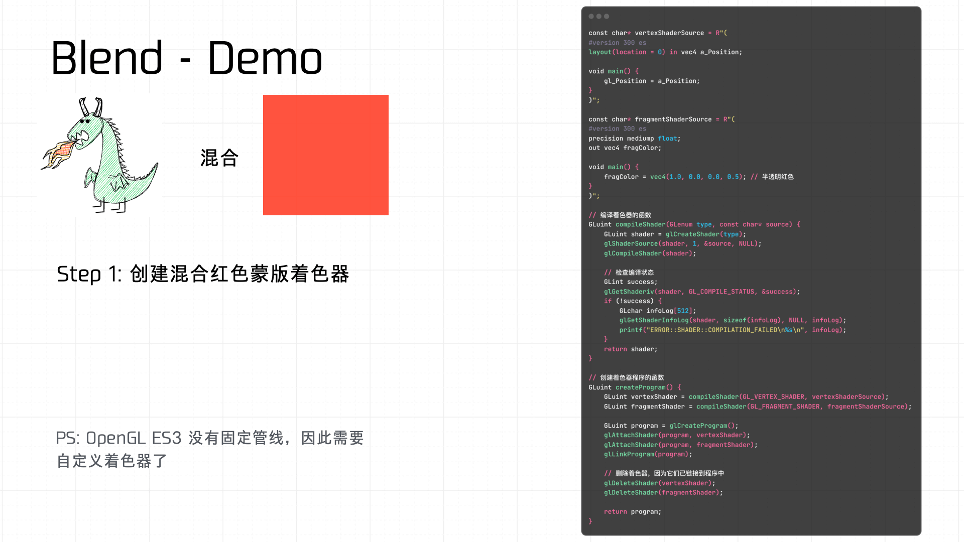
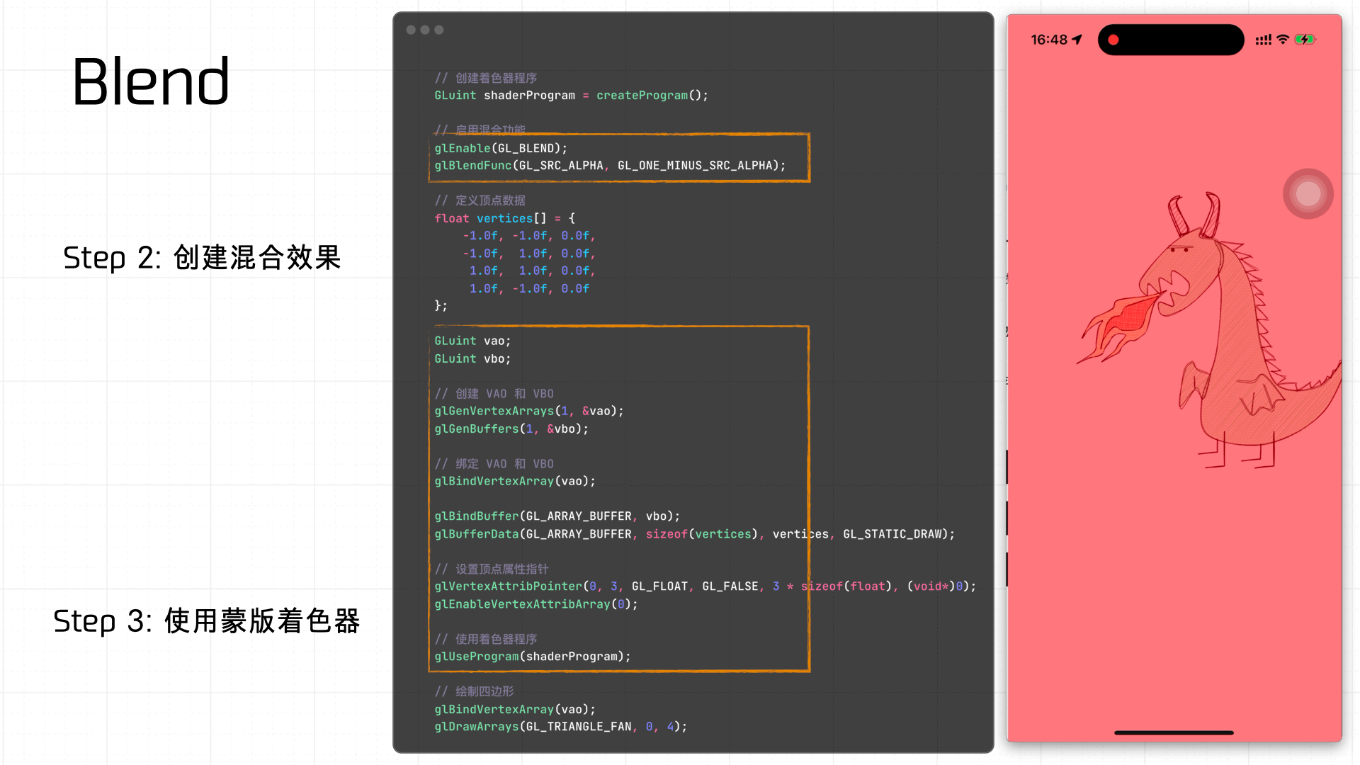
A simple example — using a shader to create a red mask Blend effect:
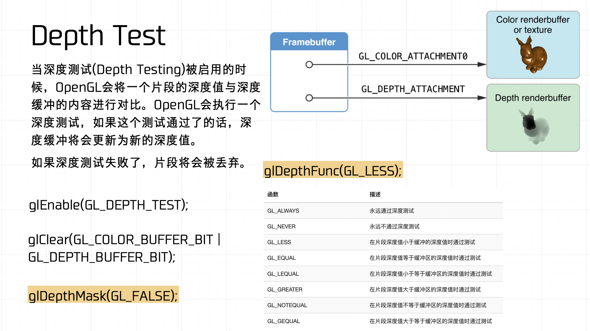
Depth Test determines whether each pixel is displayed. When depth testing is enabled, OpenGL compares the current fragment’s depth value against the depth buffer. If the fragment passes the test, the depth buffer updates to the new depth value; otherwise the fragment is discarded. Common depth test functions in OpenGL:
Stencil Test restricts the render area. Through the stencil buffer, you can create special region markers during rendering — only fragments that satisfy the stencil buffer’s conditions get rendered to screen. The stencil buffer enables complex effects like shadows, mirror reflections, and outline highlights. Common stencil test functions in OpenGL:
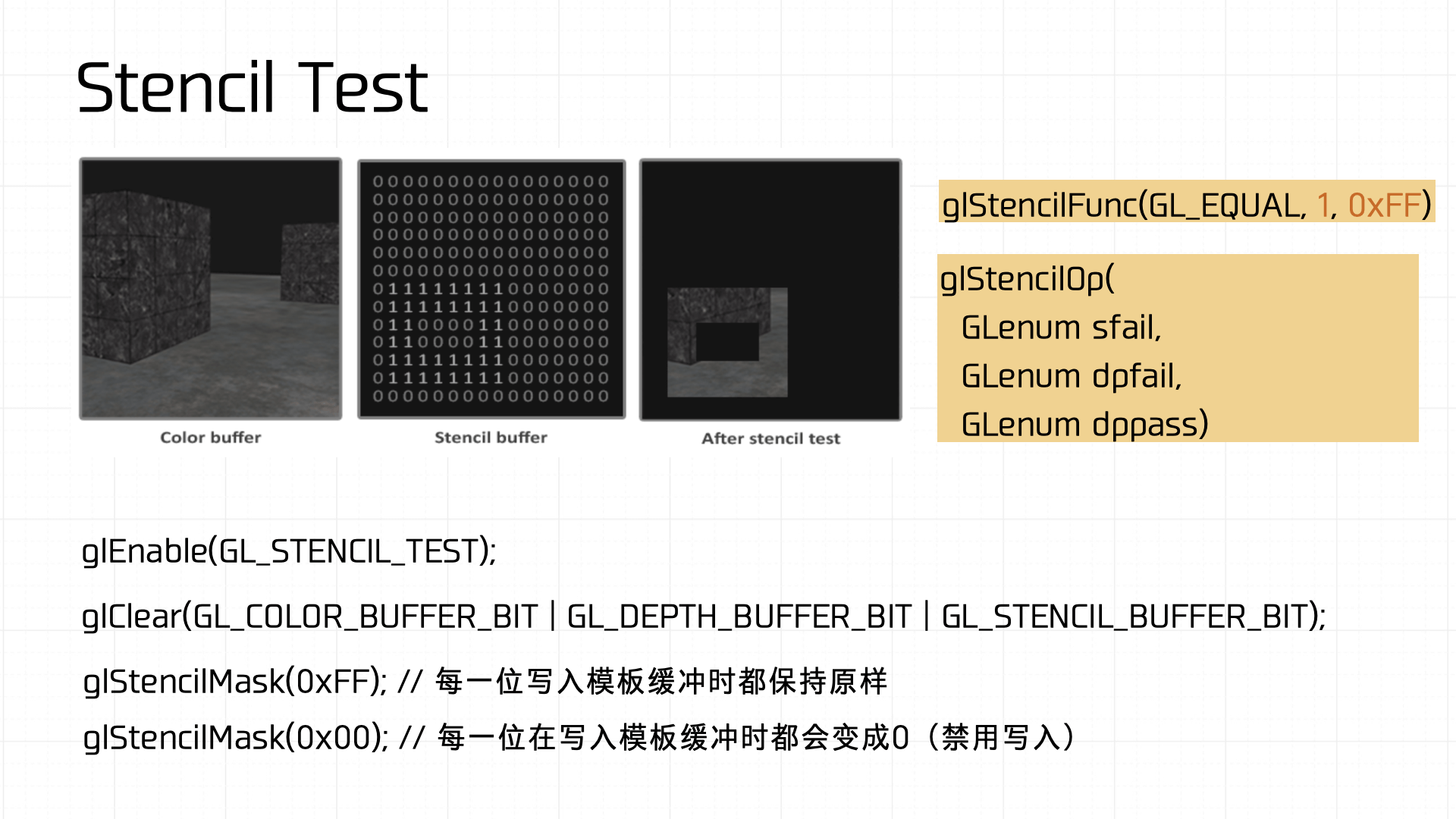
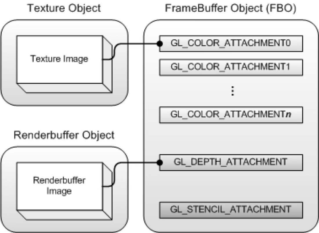
All of these results tie back to the Framebuffer’s Attachment mechanism, which determines how render results are written to the buffers. A Framebuffer typically carries multiple buffers — the color buffer (GL_COLOR_ATTACHMENT), depth buffer (GL_DEPTH_ATTACHMENT), and stencil buffer (GL_STENCIL_ATTACHMENT) — which together determine the final rendered output.
3.10 Commit & Draw Pass
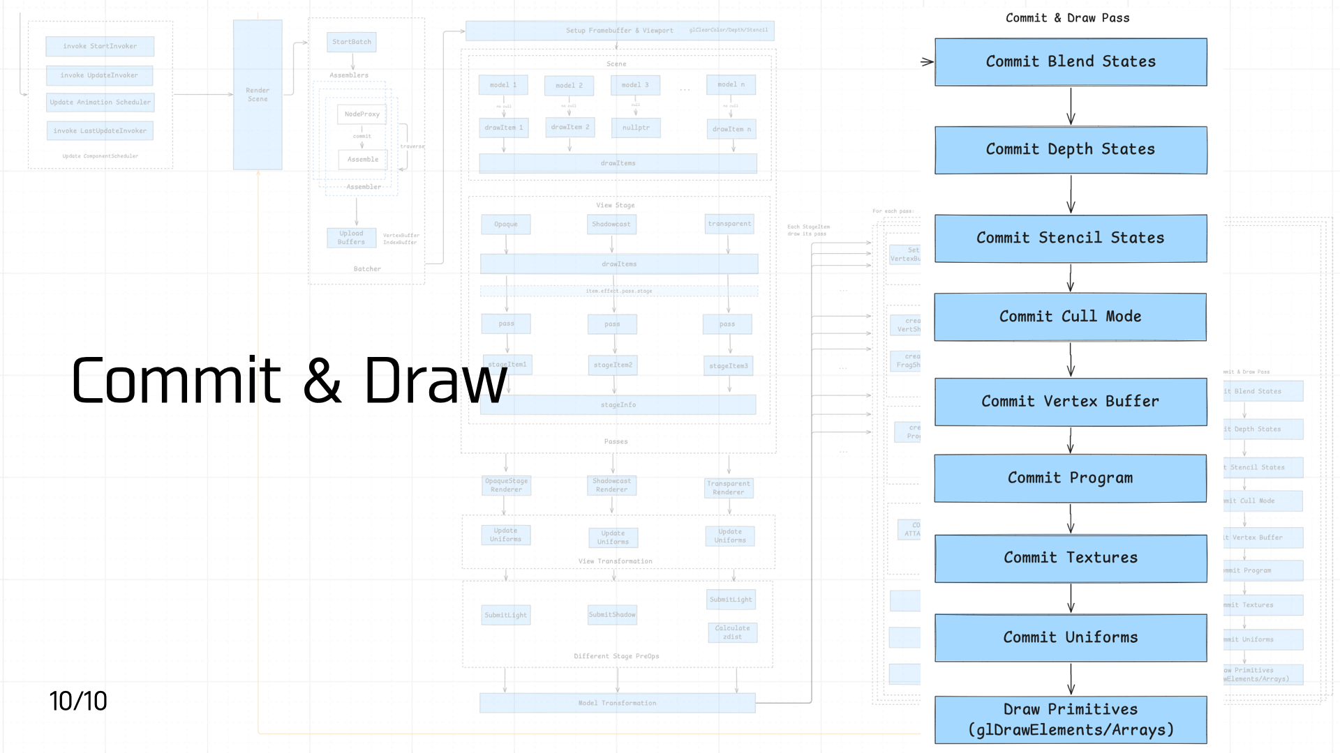 The final stage in the pipeline: Commit and Draw.
In Cocos, each frame stores two states: the current frame state (currentState) and the upcoming render frame state (nextState).
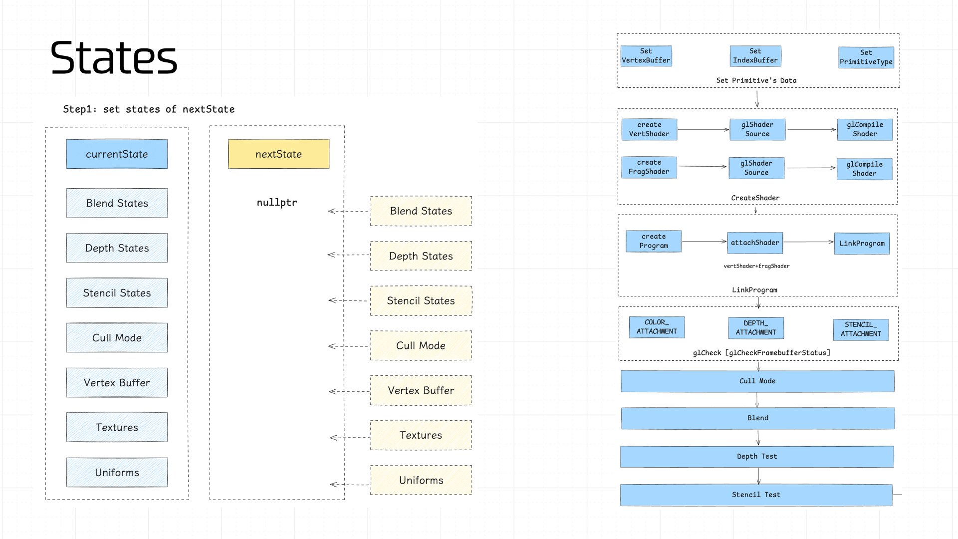
We compute each component of nextState in sequence, then diff nextState against currentState. If any stage’s state value differs, a commit operation is triggered — allowing the pipeline to maximize cache reuse.
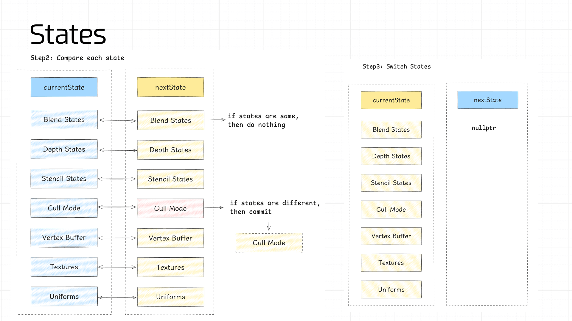
The state values managed in the pipeline:
- Blend States, Depth States, Stencil States
- Cull Mode
- Vertex Buffer
- Program
- Textures
- Uniforms
Note: the Program is typically prepared for all shaders during pipeline initialization; under normal conditions its cache never invalidates, so it’s not shown in the diagram above.
Blend States, Depth States, and Stencil States store the GL call parameters and partial results from the Blend, Depth Test, and Stencil Test stages described earlier — no need to expand on those here.
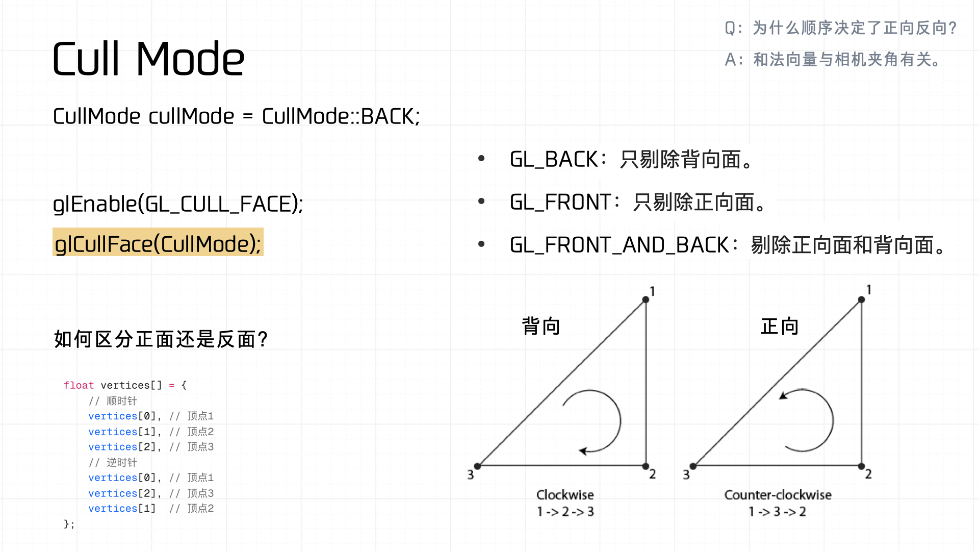
Next is Cull Mode — uses vertex index winding order (clockwise vs counterclockwise) to distinguish front from back faces. If the state differs from currentState, glCullFace is called to commit:
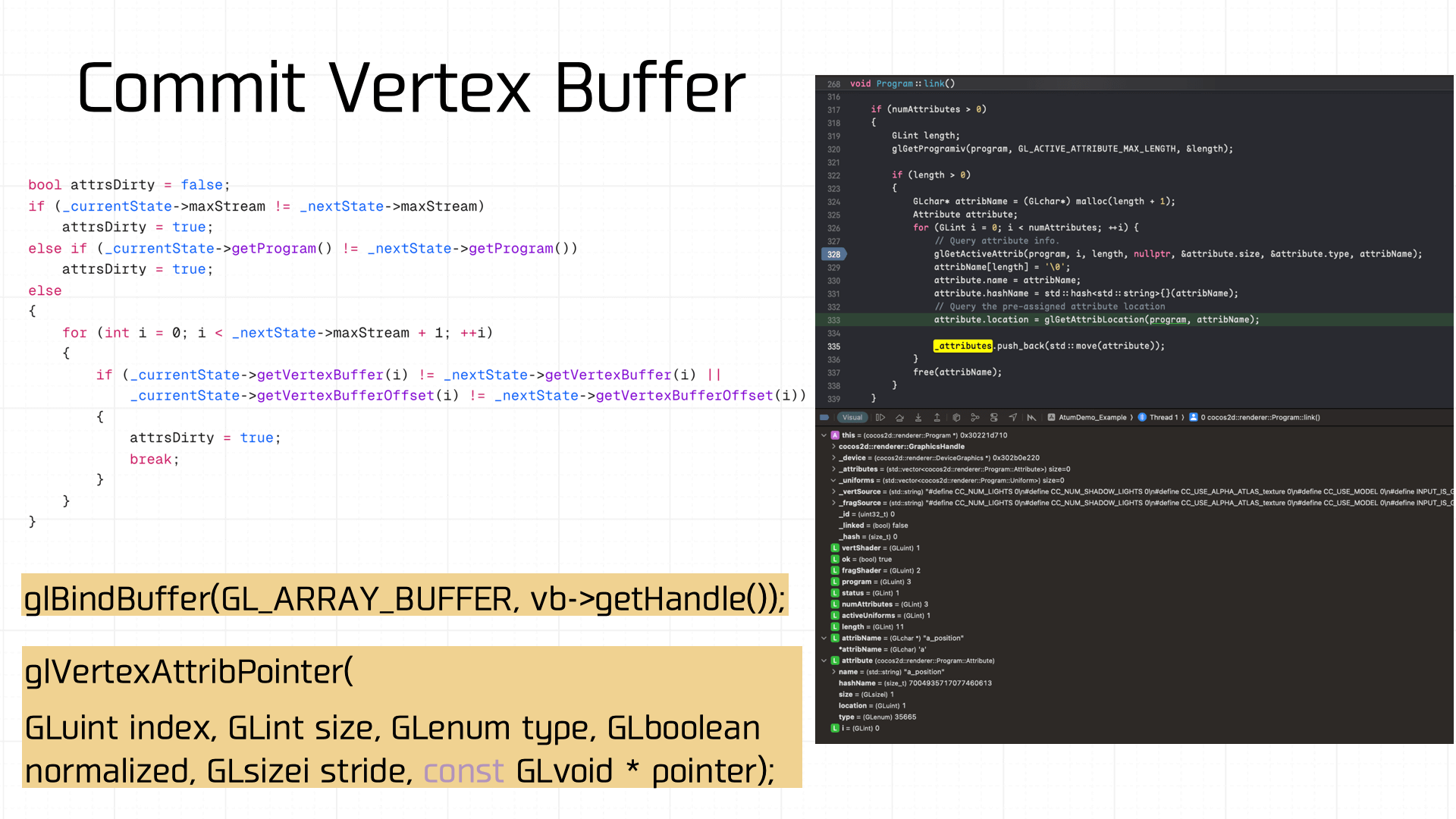
The Vertex Buffer also has state management. If it’s dirty, glBindBuffer is called to rebind:
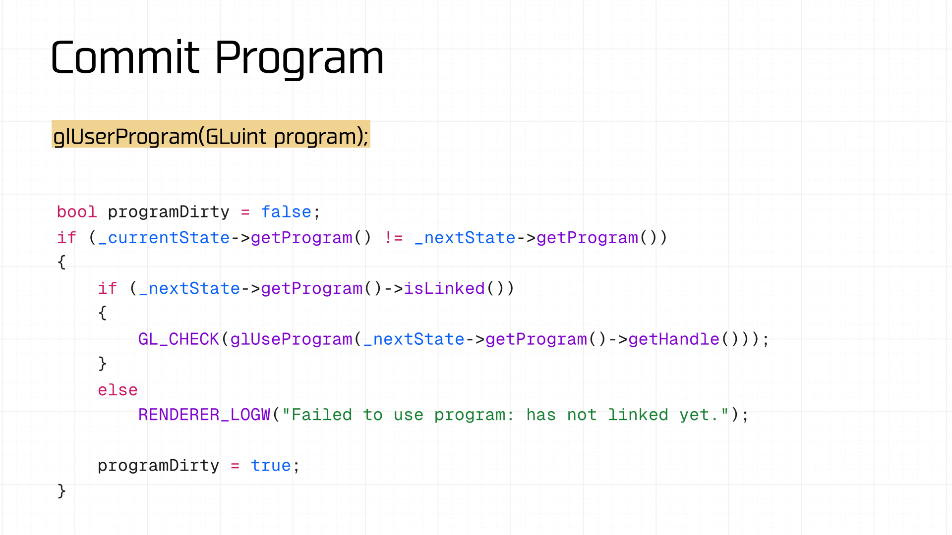
The shader program is the same — if dirty, glUseProgram is called to reset it:
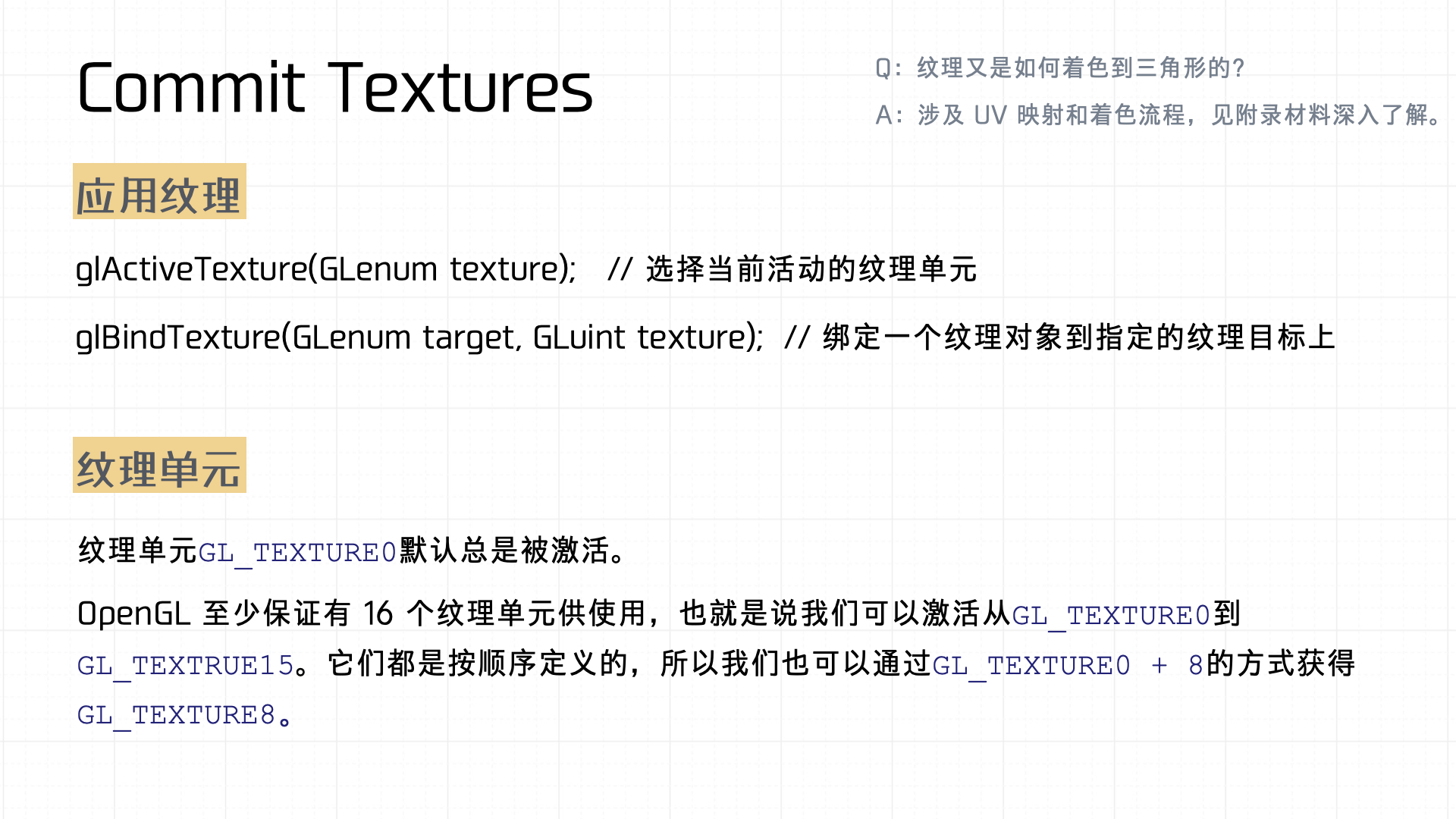
Then Textures are checked and committed. Two key points:
- Texture activation: Involves
glActiveTextureandglBindTexture. First,glActiveTextureselects which texture unit to activate — determining which unit the subsequently bound texture will act on. ThenglBindTexturebinds a specific texture object to a particular texture target. This mechanism associates texture objects with texture units and targets, completing texture activation and binding. - Texture units: Represent the multiple textures a GPU can manage simultaneously. By default,
GL_TEXTURE0is always active. OpenGL guarantees at least 16 texture units (GL_TEXTURE0throughGL_TEXTURE15). Since they’re defined sequentially, you can access a specific unit conveniently with expressions likeGL_TEXTURE0 + 8, enabling multiple textures in complex rendering scenarios.
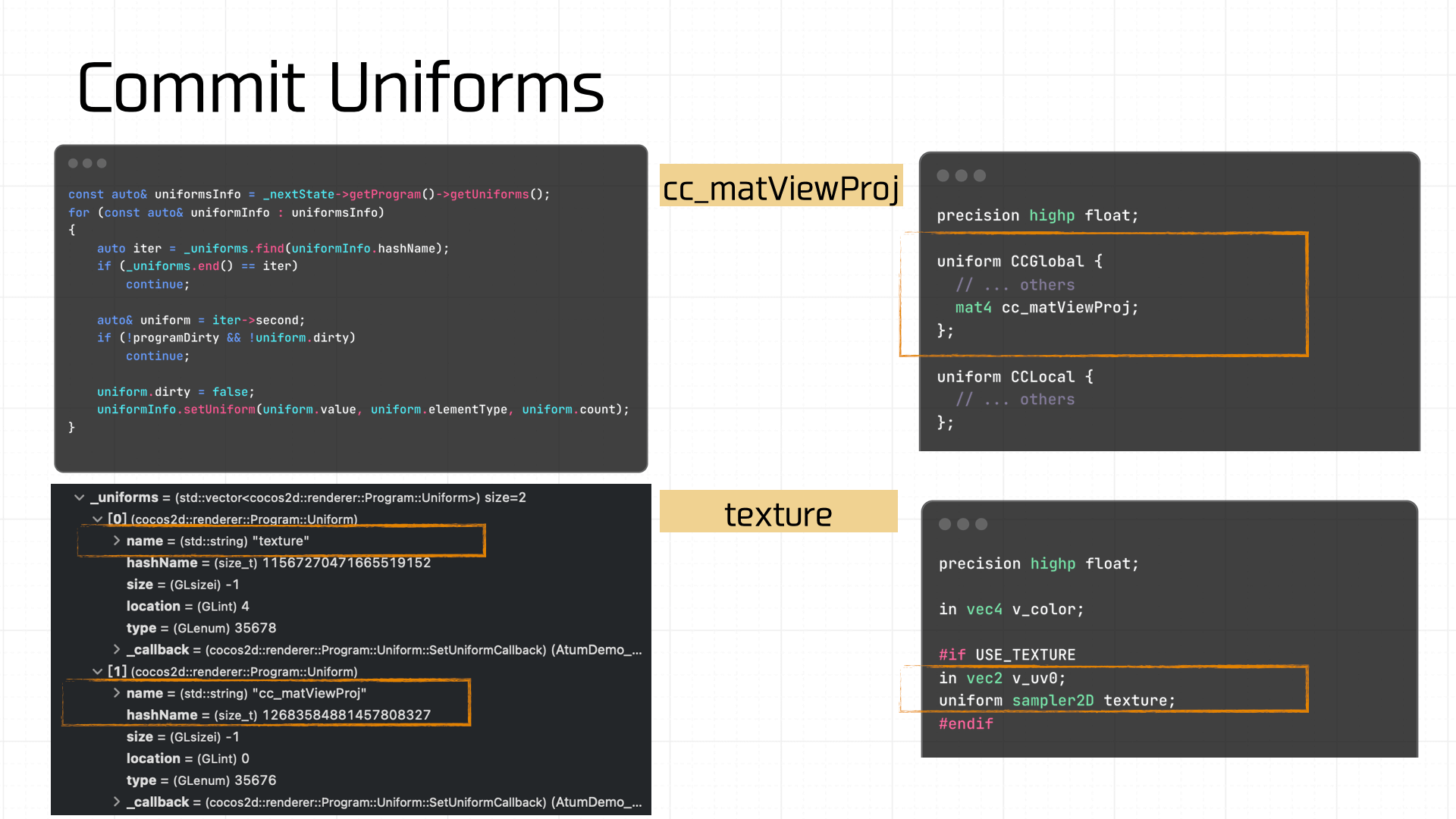
Once the preceding state values are prepared and committed, the final state to manage is Uniforms. If this is dirty, the Uniform variables must also be resubmitted. In our demo, the Uniform variables involved are cc_matViewProj and texture:
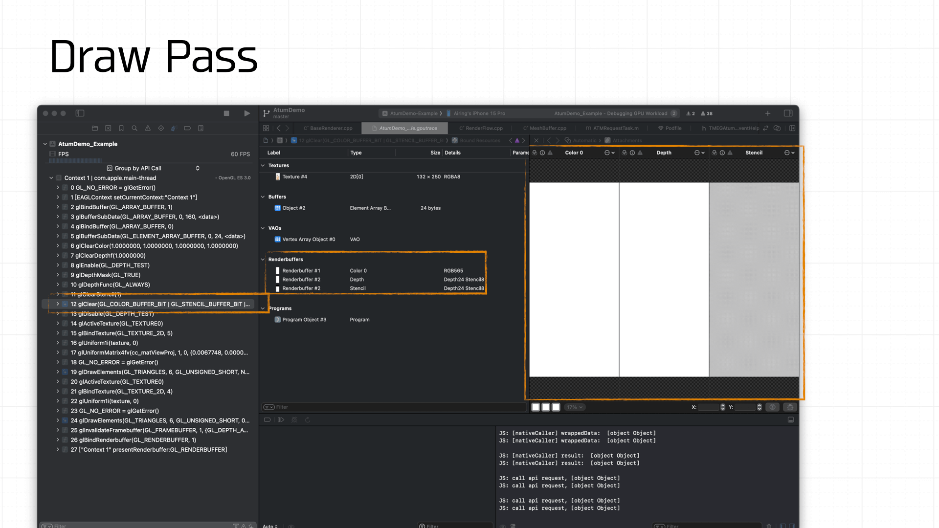
Finally, the Draw. Before drawing each frame, glClear must be called to clear the Framebuffer state. The diagram below shows the timing sequence of GL command calls:
Because the demo is simple, drawing only requires the texture and Uniforms to be ready. The final call is glDrawArrays or glDrawElements to draw the prepared Framebuffer onto the screen:
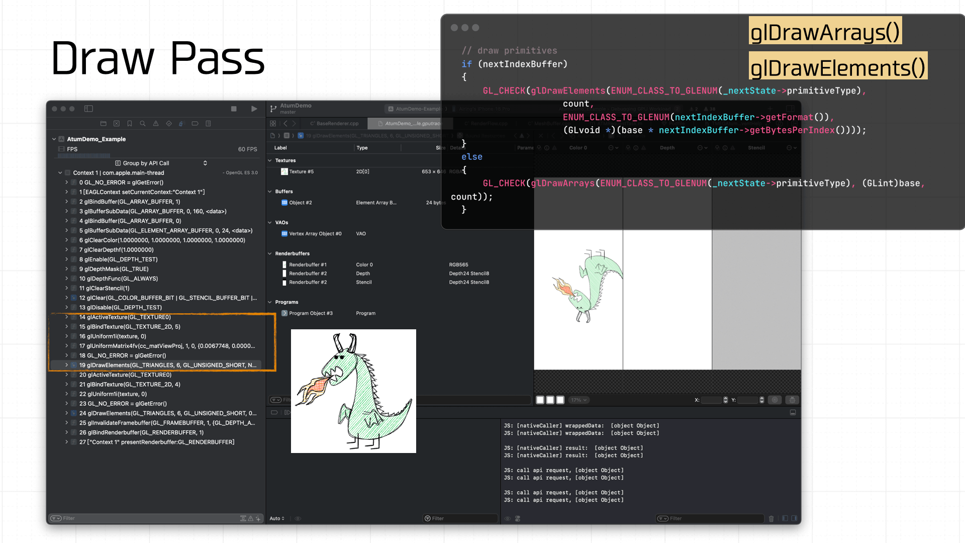
And with that, after traversing the entire pipeline, our demo game has completed its journey to the screen inside the mini-game container.
Further Reading
- GAMES 101
- Introduction to Computer Graphics: A Guide to 3D Rendering
- LearnOpenGL (Chinese: LearnOpenGLCN)