Abstract: This paper discusses how to construct a complete intelligent learning system in an online learning space from five dimensions. In addition to an overall architectural design, it provides systematic scientific analysis and code implementation for data storage, learner modeling, and knowledge modeling. In the final push algorithm analysis, the above modules are consolidated, deriving algorithms including Dijkstra, UserCF, ItemCF, and CAS. After implementing each algorithm and evaluating performance with Top-N, the system is re-optimized to produce a high-performance, highly applicable push algorithm. The adaptive intelligent learning system built around this algorithm constitutes a complex educational ecosystem with characteristics of intelligent flexibility, balance and harmony, and sustainable development. Only such an algorithm can be considered a genuine learning community.
Keywords: intelligent learning system, recommendation algorithm, learner modeling, knowledge network
ABSTRACT: This paper mainly discusses how to construct a kind of intelligent learning system under the network learning space from five aspects. It not only constructs the design from the whole, but also carries on the scientific system to the data storage, the learner modeling and the knowledge analysis and code implementation. In the final push algorithm analysis, the above modules are summarized, which derived Dijkstra, UserCF, ItemCF, CAS and other algorithms, the implementation of various algorithms, and the use of Top-N performance evaluation, re-optimization, which to achieve a high-performance, high applicability of the push algorithm. The adaptive intelligence learning system, which is based on the algorithm, is a complex educational ecosystem with intelligent and flexible, balanced and harmonious and sustainable development. Only one such algorithm can be regarded as a real learning community.
KEY WORDS: intelligent learning system, recommendation algorithm, learner modeling, knowledge network
1. Introduction
1.1 Background
This paper, titled “Research on an Intelligent Push System for Online Learning Resources,” aims to design an adaptive intelligent learning system with a focus on its push algorithms. The goal is to enable the intelligent learning system to “intelligently” push learning resources to learners, breaking the previous pattern of learners searching for educational information blindly and sporadically. Instead, educational information should actively find the right learner — proactively, personally, intelligently, and efficiently [1].
This research spans the domains of education, computer science, and mathematical-statistical analysis. In education, the subject is the student and the object is educational information resources (the knowledge network). In mathematical statistics, the key challenge is modeling both subject and object, with the core difficulty being the development of a recommendation algorithm through which the object actively selects the subject. In computer software, the foundation is system construction, algorithm implementation, and testing and application.
The key technologies in this research have been implemented in their respective domains, but intelligent push specifically — the core of the system — has not been applied in education. The reason is that “knowledge modeling” research is still in its early stages, with no unified standard domestically or internationally [35]; learner modeling methods are also highly varied with no consensus. In the pure recommendation systems field, item [10] provides a comprehensive summary of excellent algorithms. Large internet platforms — Amazon abroad, Meituan in China — have designed their own high-performance recommendation systems. In machine learning and statistics, various clustering and association algorithms exist — yet none of these have been proposed for use in intelligent learning systems. This represents a cross-disciplinary gap and a gap in the education field. This research focuses precisely on exploring and refining “knowledge modeling,” improving “learner modeling” methods, and integrating and optimizing existing recommendation algorithms to implement an intelligent push system in the education domain.
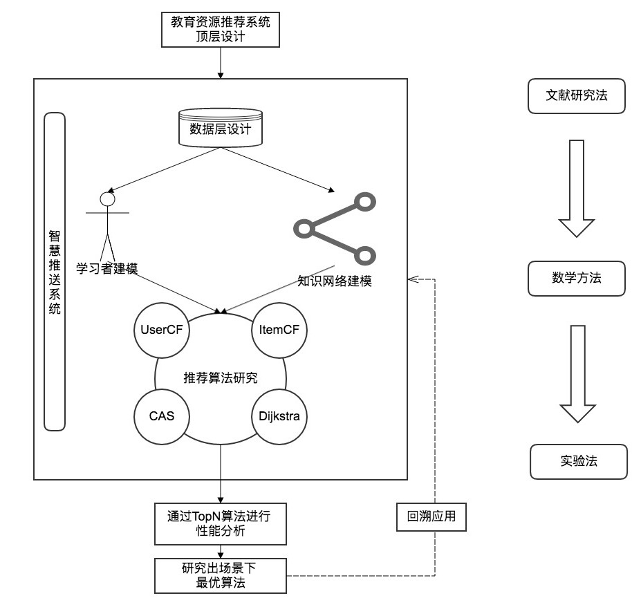
This paper discusses the construction of a complete networked intelligent learning system (Figure 1) from five dimensions: overall architectural design, data storage, learner modeling, knowledge modeling, and push algorithm analysis. Algorithms including Dijkstra, UserCF, ItemCF, and CAS are derived; Top-N is used for performance evaluation and re-optimization, yielding a high-performance, highly applicable push algorithm. The adaptive intelligent learning system built on this algorithm is a complex educational ecosystem with intelligent flexibility, balance and harmony, and sustainable development [8].
1.2 Domestic and International Context
With the rapid development of internet technology, new technologies continue to emerge one after another — intelligent learning is one of them. Informatization has greatly changed how people learn. Student-centered, differentiated instruction is increasingly tailored to the individual: learning activities are becoming more personalized, more dependent on digital environments, more ubiquitous, and the attributes of learning environments and resources are increasingly resembling consumer products [6].
MBAlib defines intelligent learning as a learning process in which learners in a smart environment access learning resources on demand, flexibly carry out learning activities, and quickly build knowledge networks and interpersonal networks. The ultimate goal of intelligent learning is to develop learners’ learning wisdom and improve their creative capacity — a new mode of learning that has evolved from e-learning, mobile learning, and ubiquitous learning under the guidance of smart education philosophy.
In a 2013 paper [16], Korean scholar Hwang defined “smart learning” as a relatively flexible form of learning that enhances learner capabilities through the use of open educational resources, smart information technology (Smart IT), and international standards. In the same year [4], another paper explored the evolution of intelligent learning in depth: “intelligent learning” allows people to focus more energy on learning topics, seamlessly accessing a mobile ubiquitous learning space through various smart terminal devices, flexibly customizing and transparently accessing the most appropriate and convenient resource services, enabling self-directed active learning.
Surveying the domestic literature, scholars have mostly stayed at the conceptual level. Even where models have been proposed, these are typically modeling studies of individual recommendation system components, without algorithmic or feasibility analysis — and thus incomplete.
The 2016 paper [5] studied learning behavior analysis and recommendation systems in smart learning spaces, proposing a learning recommendation mechanism, modeling learners, conducting a data-layer design, and applying collaborative filtering and ant colony algorithms to the recommendation system. This is one of the more complete designs, but the algorithmic research is not thorough: only the ant colony algorithm is analyzed in detail, with no performance evaluation, no study of user collaborative filtering, no holistic system modeling, and no knowledge network modeling. The data layer is mentioned but lacks implementation technology.
These gaps in algorithm and technology in intelligent learning systems can be partially explained by the educational context. In the pure recommendation systems field, comprehensive algorithm collections exist, such as those summarized in [10]. Large internet platforms have developed efficient, high-quality recommendation systems. Machine learning and statistics offer clustering and association algorithms — yet none of these have found their way into intelligent learning systems. This is the cross-disciplinary shortcoming and the regret of the education field.
2. Top-Level Design of the Intelligent Learning System
2.1 System Overview
Synthesizing domestic and international definitions, we can define an intelligent learning system as: a seamless system in which knowledge resource objects actively seek out learning-activity subjects.
Educational data is extensive; the learning process is adaptive. Given these properties, the intelligent learning system should be grounded in learning analytics technology and centered on push technology. Through the online learning platform environment, it should mine and analyze educational data to provide learners with feedback that improves learning behavior. Concretely: mine behavioral data through the online learning platform’s big data, identify which behaviors to analyze, then perform learner behavior modeling, learner experience modeling, and learner knowledge modeling. Apply the mined and cleaned data to these models and, leveraging the system’s early-warning and predictive capabilities, analyze learner learning trends and develop intervention modules to adaptively adjust learning content and behavior, optimize learning paths, and strengthen learning efficiency and deepen knowledge structure. Most critically, through the improved and optimized recommendation algorithm, achieve “intelligent push of learning resources” personalized to each individual — thereby realizing the full value of the intelligent learning system.
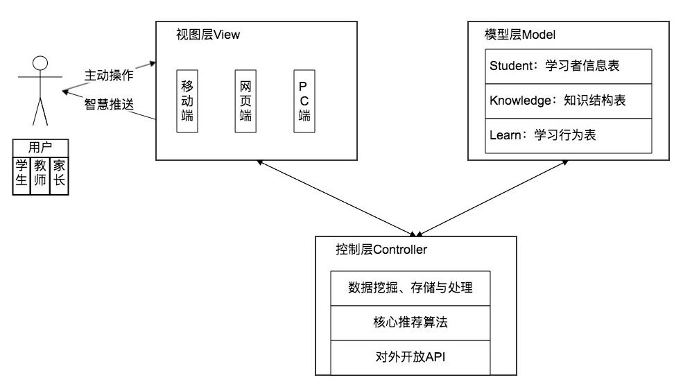
Based on this, the intelligent learning system architecture is designed as shown below. The entire system is based on the MVC model. The View Layer is the online learning platform, based on current network spaces — including mobile, web, and PC — directly interacting with users, who include students, parents, and teachers. The Model Layer is the system database, storing learner basic information, knowledge point information, and learning behavior data. The Control Layer is the system hub, providing data analysis and recommendation algorithms, pushing data to the View Layer and forwarding data to the Model Layer.
2.2 Intelligent Push Flow Overview
Intelligent push works by matching learner behavioral data with knowledge point data in the database. The key emphasis is on learner feature modeling. If data reliability is insufficient for matching and modeling, the scope and intensity of data mining must be expanded until sufficient to support precise recommendations. After recommending the next knowledge point, the learner studies accordingly, and the data mining system can further mine learning data to better support the algorithm. This closed-loop recommendation system makes pushes increasingly precise and learning increasingly efficient — a virtuous cycle beneficial to both sides.
st=>start: Start
e=>end: End
op1=>operation: Use system to learn
op2=>operation: System collects and analyzes data
sub1=>subroutine: Expand collection scope
cond=>condition: Meets minimum algorithm
requirements?
op3=>operation: Recommend next knowledge point

st->op1->op2->cond
cond(yes)->op3->op1
cond(no)->sub1(right)->op2
2.3 Data Layer Design
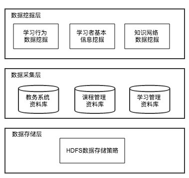
2.3.1 Overall Data Layer Design
The intelligent learning system is grounded in data — without data, there is no algorithm. The data layer design is therefore especially important.
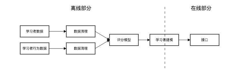
The system subdivides the data layer into three parts: data mining layer, data collection layer, and data storage layer. The data mining layer includes learning behavior data mining, learner basic information mining, and knowledge network data mining. The data collection layer encompasses educational affairs databases, curriculum management databases, and learning management databases. The data storage layer applies Hadoop’s HDFS data storage strategy for efficient and secure large-volume storage of learner feature information, knowledge network information, and learning behavior information.
2.3.2 Data Mining and Collection Layer Design
Based on a learning behavior extraction matrix referenced from [8], and adapted to the characteristics of the intelligent learning system, learner behaviors in the system include creation, annotation, sharing, selection, use, and retention. Corresponding functions are retrieved, and implicit data is mined and collected from the educational affairs, curriculum management, and learning management databases for storage. The new learning behavior extraction matrix essentially represents mining of dynamic information data.

2.3.3 Data Storage Layer Design
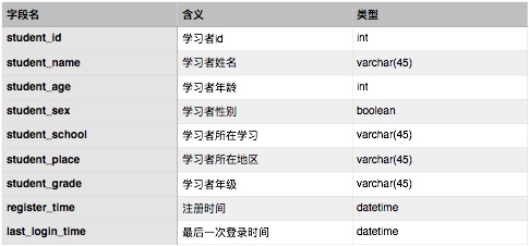
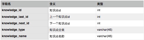
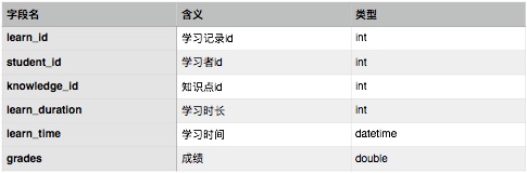
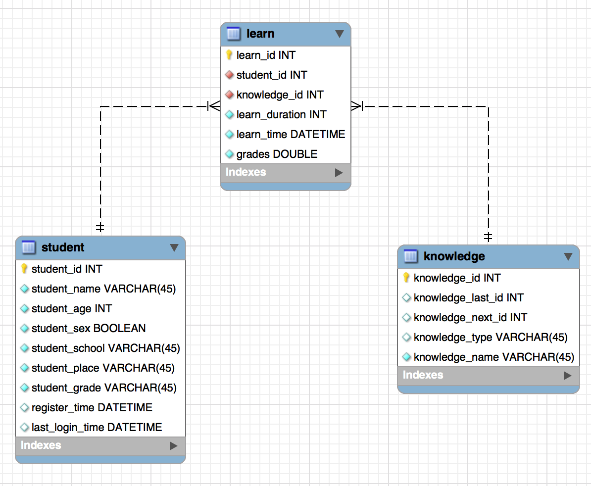
The storage layer requires three modules to store three categories of data: learner data, knowledge point data, and learning behavior data. Three corresponding tables are designed, with fields representing basic system information that can be extended as needed.
Learner information table:
Knowledge point information table:
Learning record table:
The E-R diagram of the above table models:
For data storage, a disaster recovery mechanism is essential. Here we adopt HDFS storage strategy: stored data is split into n blocks, each with 3 replicas, distributed across 3 nodes in 2 racks (2 replicas on rack 1, 1 on another rack). If any node fails, a backup can be retrieved from another node on the same rack, or from another rack if the fault is more serious.
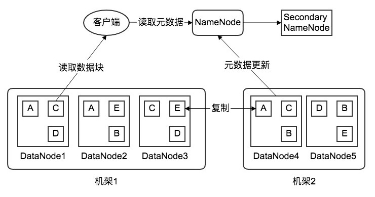
Each DataNode sends regular heartbeat checks to the NameNode reporting its status. Through this heartbeat protocol, the NameNode can monitor the entire cluster’s operational state. The Secondary NameNode periodically synchronizes metadata image files and edit logs; when the NameNode fails, the Secondary NameNode takes over to ensure normal cluster operation and high system availability.
2.3.4 Data Flow Processing
As shown above, the intelligent learning system generates large volumes of data, and the push system requires high efficiency and real-time performance — creating extreme requirements for data stream processing. If real-time and efficiency requirements are not met, educational resources cannot be precisely and timely pushed to learners, causing lag in learning behavior. Intelligent learning systems represent a new frontier of educational informatization development, and realizing this goal requires efficient learning analytics technology [9] — essentially, efficient learning data stream processing.
MapReduce is a big data processing solution worth considering here — a divide-and-conquer approach applied to data processing. MapReduce divides a large task into subtasks (Map phase), executes them in parallel, then merges the results (Reduce phase) [31].
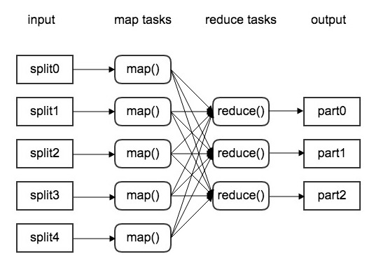
In the Map phase, data is read from text files, tables, databases, etc. — the behavioral data continuously generated by the intelligent learning system. These potentially massive numbers of files (called shards) are treated as a logical input source, then processed independently and in parallel by a user-implemented function called a Mapper. For each shard, the Mapper returns multiple key-value pairs — the Map phase output.
Between Map and Reduce is a Shuffle phase: key-value pairs are grouped by key. The output is a stream of distinct keys paired with their associated values.
In the Reduce phase, the Shuffle output is processed by a user-implemented function called a Reducer, independently and in parallel for each distinct key and its associated value stream. Each Reducer iterates over the values for each key, “transforms” them (usually aggregating), and writes key-value pairs to the database.
Through MapReduce, large-scale data can be processed efficiently — fully applicable to the intelligent learning system’s demanding data stream requirements.
3. Learner Feature Analysis and Modeling
3.1 Overview
For push problems, data alone is not sufficient. Extracting meaningful patterns from complex data requires appropriate analytical methods — for example, clustering analysis. Applying clustering algorithms to appropriately group data, building learner models based on each group’s characteristics, and enabling more precise educational resource recommendations.
st=>start: Start
e=>end: End
op1=>operation: Learner cluster analysis
op2=>operation: Learner feature construction and selection
op3=>operation: Learner modeling and optimization
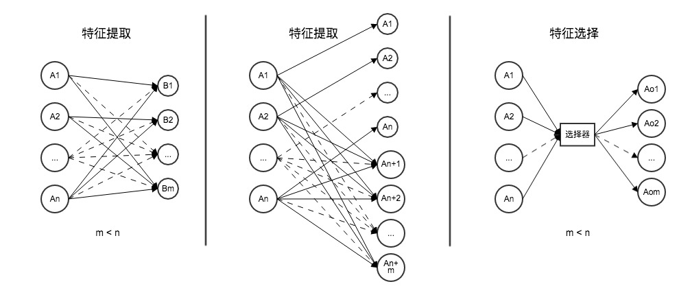
st->op1->op2->op3->eFeatures are critical for precise recommendation. Most pre-modeling work is devoted to finding features. Without appropriate features, learner models are essentially guesswork and serve no purpose in an intelligent learning system. Features are the interesting variables or attributes in input data that noticeably affect the dependent variable. The three main feature analysis methods are: feature extraction (mapping original features to new features via a function), feature construction (inferring or building additional features from original features), and feature selection (selecting m (m<n) optimal features from the original n features to achieve optimal simplification and dimensionality reduction). Since raw data in the intelligent learning system is large-scale, incomplete, and implicit, feature extraction is inappropriate; feature construction and selection are the appropriate approaches.
3.2 Learner Cluster Analysis
Cluster analysis groups learners by similarity, building learner populations across different levels and domains. Since learner attributes span many dimensions, the system should use hierarchical clustering rather than the K-Means algorithms mentioned in some domestic research.
Hierarchical clustering starts with each sample as its own class. Under a defined inter-class distance measure, the two classes closest to each other merge into a new class, and their distance to other classes is recalculated. This continues — one fewer class per iteration — until all samples form a single class. The algorithm:
op1=>operation: Each sample forms its own class
op2=>operation: Compute inter-class distance matrix
op3=>operation: Merge two nearest classes into new class
cond=>condition: Number of classes = 1?
op4=>operation: Draw dendrogram
op5=>operation: Determine cluster count and memberships

op1->op2->op3->cond
cond(yes)->op4->op5
cond(no)->op2
The table below shows a worked example using 6 learners across 5 behavioral dimensions, with Euclidean distance and the nearest-neighbor method:

Step 1: Each sample forms its own class.
$G_1^{(0)}={x_1},G_2^{(0)}={x_2},G_3^{(0)}={x_3}$ $G_4^{(0)}={x_4},G_5^{(0)}={x_5},G_6^{(0)}={x_6}$
Step 2: Compute distances to get $D^{(0)}$:
$$ D^{(0)}= \begin{bmatrix} 0 & 9.540 & 8.660 & 4.900 & 4.690 & 6.780 \ 9.540 & 0 & 10.30 & 11.79 & 10.82 & 7.140 \ 8.660 & 10.30 & 0 & 11.09 & 9.330 & 10.15 \ 4.900 & 11.79 & 11.09 & 0 & 6.480 & 5.830 \ 4.690 & 10.82 & 9.330 & 6.480 & 0 & 8.120 \ 6.780 & 7.140 & 10.15 & 5.830 & 8.120 & 0 \ \end{bmatrix} $$
Step 3: Minimum element is 4.690 (between $G_1^{(0)}$ and $G_5^{(0)}$). Merge them: $G_1^{(1)}={x_1,x_5}$, etc.
Step 4: Recompute $D^{(1)}$:
$$ D^{(1)}= \begin{bmatrix} 0 & 9.540 & 8.660 & 4.900 & 6.780 \ 9.540 & 0 & 10.30 & 11.79 & 7.140 \ 8.660 & 10.30 & 0 & 11.09 & 10.15 \ 4.900 & 11.79 & 11.09 & 0 & 5.830 \ 6.780 & 7.140 & 10.15 & 5.830 & 0\ \end{bmatrix} $$
Step 5: Minimum is 4.900 (between $G_1^{(1)}$ and $G_4^{(1)}$). Merge them: $G_1^{(2)}={x_1,x_4,x_5}$
Step 6: Recompute $D^{(2)}$:
$$ D^{(2)}= \begin{bmatrix} 0 & 9.540 & 8.660 & 5.830 \ 9.540 & 0 & 10.30 & 7.140 \ 8.660 & 10.30 & 0 & 10.15 \ 5.830 & 7.140 & 10.15 & 0 \ \end{bmatrix} $$
Step 7: Minimum is 5.830. Merge $G_1^{(2)}$ and $G_4^{(2)}$: $G_1^{(3)}={x_1,x_4,x_5,x_6}$
Step 8: Recompute $D^{(3)}$:
$$ D^{(3)}= \begin{bmatrix} 0 & 7.140 & 8.660 \ 7.140 & 0 & 10.30 \ 8.660 & 10.30 & 0 \ \end{bmatrix} $$
Step 9: Minimum is 7.140. Merge $G_1^{(3)}$ and $G_2^{(3)}$: $G_1^{(4)}={x_1,x_2,x_4,x_5,x_6}$
Step 10: Two classes remain — merge into one final class.
Clustering of learners by learning behavior is complete.
3.3 Feature Construction and Selection
3.3.1 Feature Construction
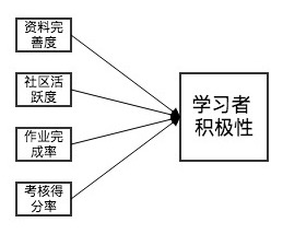
Feature construction uses two main methods: feature transformation and feature combination. Feature transformation derives new features from originals via a rule or mapping. For example, using concept hierarchies, 6 learners at grade levels 7, 8, 10, 11, junior 3, and senior 3 can be grouped into three categories: middle school, high school, university. Feature combination derives new features from two or more originals, such as combining profile completion rate, community activity, assignment completion, and test scores to produce a “learner engagement” feature with better discriminative power.
For the intelligent learning system, feature construction is best done manually by domain experts in educational analytics, who study the data from pilot runs and combine their domain knowledge to transform and combine features into more discriminative ones.
3.3.2 Feature Selection
After feature construction, the dataset still contains many features, some correlated and some redundant. To improve modeling efficiency and obtain better discriminative features, dimensionality reduction is needed to find an optimal subset — the process of feature selection.
The Gini coefficient measures inequality. In a classification problem, the Gini coefficient of a classification node A represents the probability that a sample is misclassified in its subset. It is computed as the probability of a sample being selected ($p_i$) multiplied by the probability of misclassification ($1-p_i$). With $k$ classes and $p_i$ as the probability a sample belongs to class $i$:
$Gini(A) = \sum_{i=1}^k p_i(1-p_i) = 1 - \sum_{i=1}^k p_i^2$
Example: 10 students, features X1 (homework completed: yes/no), X2 (learning frequency: low/medium/high), and outcome Y (course assessment passed: yes/no).

Step 1: Compute Gini for X1 vs Y.

$Gini(X1 = \text{No}) = 1 - ({2\over5})^2 - ({3\over5})^2 = 0.48$
$Gini(X1 = \text{Yes}) = 1 - ({5\over5})^2 - ({0\over5})^2 = 0$
$Gini(X1) = {5\over10} \cdot 0.48 + {5\over10} \cdot 0 = 0.24$
Step 2: Compute Gini for X2 vs Y.
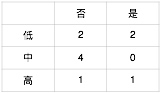
$Gini(X2 = \text{Low}) = 0.5$, $Gini(X2 = \text{Medium}) = 0$, $Gini(X2 = \text{High}) = 0.5$
$Gini(X2) = {4\over10} \cdot 0.5 + {4\over10} \cdot 0 + {2\over10} \cdot 0.5 = 0.3$
Step 3: Since $Gini(X2) > Gini(X1)$, feature X1 is more important than X2. Whether homework was completed matters more than learning frequency for assessment success. Similarly, all features can be ranked by Gini coefficient and redundant ones filtered out.
3.4 Learner Persona and Modeling
Feature construction and selection allow us to build a learner persona. For the intelligent learning system, key technical challenges in persona construction include: continuously optimizing the algorithmic model; introducing real-time technologies like Storm; supplementing with new tag types including topic recommendation tags and named entity recognition; separating offline and online HBase reads, separating KV reads from Solr batch reads, monitoring and splitting HBase region hotspots; continuously optimizing data flow; and improving data storage [26].
The root causes are large data volumes, computational complexity, and high real-time requirements. A relatively simple solution is offline/online separation of HBase to improve availability. A sample model:
The entire system is data-driven: by studying data, continuously generating updated learner personas and optimizing learner models. The most important part of optimizing the learner model is optimizing model parameters to obtain better models.
3.5 Model Parameter Optimization
Options include cross-validation, genetic algorithms, particle swarm optimization, and simulated annealing. Grid search is too computationally expensive.
3.5.1 Cross-Validation
The idea is to split learner data into N parts, repeatedly using 1 part as test set and the remaining N-1 parts as training set, then applying the trained model to the test set to get an estimate. Average the N estimates for a final model quality estimate. The best-performing model’s parameters are considered optimal or near-optimal.
3.5.2 Genetic Algorithms
Genetic algorithms simulate biological evolution through natural selection — using genetic and mutation principles to develop a random global search and optimization algorithm. The research object is a population (a set of individuals — here, a class of learners). Each individual represents a solution; encoding, selection, crossover, and mutation operations are applied iteratively to evolve toward a globally optimal solution.
op1=>operation: Generate initial population
op2=>operation: Compute fitness
cond=>condition: Optimization criterion met?
op3=>operation: Selection
op4=>operation: Crossover
op5=>operation: Mutation
op6=>operation: Best individual

op1->op2->cond
cond(yes)->op6
cond(no)->op3(right)->op4(right)->op5(right)->op2
3.5.3 Particle Swarm Optimization
PSO simulates bird flock foraging behavior — a global random search algorithm based on swarm intelligence. Like genetic algorithms, it uses “population” and “evolution” concepts, achieving optimization through cooperation and competition. Unlike genetic algorithms, PSO treats individuals as particles in a D-dimensional search space with no mass or volume, each moving at a certain speed and converging toward the particle’s own historical best position and the population’s historical best position.
op1=>operation: Generate initial particle swarm
op2=>operation: Compute each particle's fitness
op3=>operation: Update pbest, gbest; update position and velocity
cond=>condition: Max iterations reached, or best fitness increment below threshold?
op4=>operation: Algorithm terminates

op1->op2->op3->cond
cond(yes)->op4
cond(no)->op2
In combination, these three algorithms can be selectively used in the intelligent learning system to optimize learner model parameters.
4. Knowledge Network Modeling
4.1 Overview
While learners are the target of the system, the knowledge network is its primary content. Unlike learner models, knowledge network models are predominantly built from static data, so the critical challenge is choosing appropriate models. Knowledge graphs belong to complex systems and complex networks — their structure falls within random graph theory. The regularity within a domain and the randomness across domains are both prominent structural features. This section considers complex network models that balance regularity and randomness: the WS small-world network model, the BA scale-free network model, and the self-organizing coupled evolution model.
4.2 Knowledge Network Model Exploration
4.2.1 WS Small-World Network Model
Knowledge network structure combines regularity and randomness. Knowledge points within the same domain are highly regular — sequential, coherent, end-to-end; knowledge points across domains are highly random — biology may have no connection to astronomy but may have subtle connections to psychology, education, mathematics, or statistics. The small-world network model combines regularity and randomness in a relatively simple way.
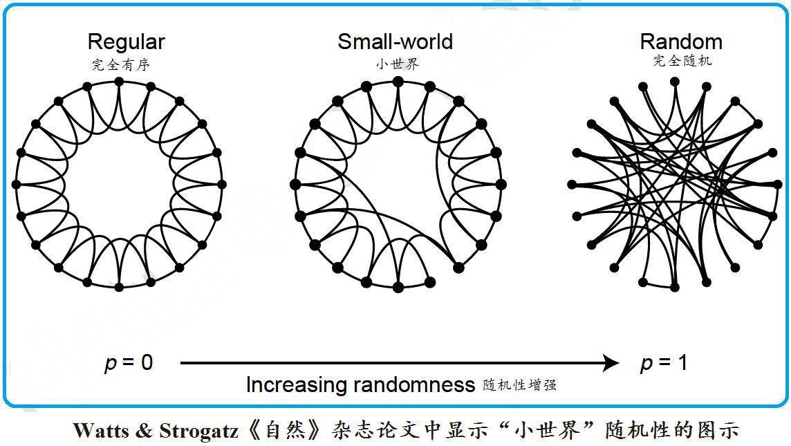
When p = 0 there are no random rewirings (regular network); when p = 1 all edges are randomly rewired (random network). Within-domain knowledge is highly regular, and there are some short-circuit paths — so the small-world model fits intra-domain knowledge networks to a degree.
4.2.2 BA Scale-Free Network Model
The small-world network’s “complexity” is a simple kind — between regularity and randomness. But the knowledge network shouldn’t be this simple or this static. Complexity should not merely sit midpoint between regularity and randomness.
We want the knowledge network model to not just have a fixed structure but also self-evolve as learner knowledge grows.
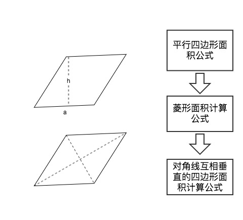
When first learning the area formula for a rhombus, learners apply the triangle area formula $S = \frac{1}{2}ah$. Later they discover that half the product of the diagonals also equals the area, and this extends to the general case of quadrilaterals with perpendicular diagonals. The knowledge network is thus extended — the learner incorporates and evolves their own knowledge framework.
The BA scale-free model incorporates two key elements: growth (the network is open; new nodes continually join) and preferential attachment (the probability of connecting to a node is proportional to its degree [34]).
The model is described as follows:
Starting at $t = 0$ with a small number $m_0$ nodes, at each time step, learning behavior data is read to add new knowledge nodes, connected to $m$ ($m \le m_0$) existing nodes.
The probability that a new node connects to existing node $i$ is proportional to $i$‘s degree, which is proportional to its confidence score: $\prod(k_i) = k_i / \sum_{j=1}^{N-1}k_j$, where $k_i$ is existing node $i$‘s confidence score and $N$ is the total node count.
This process evolves until reaching a stable state — a mature knowledge network model.
4.2.3 Self-Organizing Coupled Evolution Model
Since the knowledge network is vast and model updates require periodically scanning the entire network — a huge computational burden — a model based on local interaction mechanisms is needed to derive global network structure and properties from self-organizing dynamics. The self-organizing coupled evolution model (also called the adaptive network model) is built on ecological separation and competitive exclusion principles. It can produce changes in edge relationships from local information, leading to emergent macroscopic properties with strong plasticity. If the self-organizing coupled evolution model can be used to fit the knowledge network model, it can optimize the intelligent learning system’s performance and improve server computation efficiency. Currently, both domestic and international research on this model is still in early stages. We hope that as the theory matures, it can be applied to the intelligent learning system in practice.
4.3 Knowledge Network Association Analysis
Association analysis can uncover intrinsic rules between knowledge points from historical learning behavior data, enabling the system to make guided learning path recommendations.
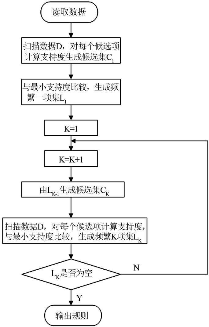
The Apriori algorithm is appropriate here. Apriori has two main steps: first, iteratively search for all frequent itemsets (sets with support no less than a set threshold); second, use the frequent itemsets to construct association rules that meet minimum confidence.
Example: 4 learners, each having studied different sets of knowledge points:
| Learner | Knowledge Points |
|---|---|
| 1 | A, C, D |
| 2 | B, C, E |
| 3 | A, B, C, E |
| 4 | B, E |
Step 1: Generate candidate 1-itemset $C_1$:
| Candidate 1-itemset | Support count |
|---|---|
| {A} | 2 |
| {B} | 3 |
| {C} | 3 |
| {D} | 1 |
| {E} | 3 |
Step 2: Min support = 2. Remove {D}. Frequent 1-itemset $L_1$:
| Frequent 1-itemset | Support count |
|---|---|
| {A} | 2 |
| {B} | 3 |
| {C} | 3 |
| {E} | 3 |
Step 3: Self-join $L_1$ to get $C_2$:
| Candidate 2-itemset | Support count |
|---|---|
| {A,B} | 1 |
| {A,C} | 2 |
| {A,E} | 1 |
| {B,C} | 2 |
| {B,E} | 3 |
| {C,E} | 2 |
Step 4: Remove {A,B} and {A,E}. Frequent 2-itemset $L_2$:
| Frequent 2-itemset | Support count |
|---|---|
| {A,C} | 2 |
| {B,C} | 2 |
| {B,E} | 3 |
| {C,E} | 2 |
Step 5: Self-join $L_2$ to get $C_3$:
| Candidate 3-itemset | Support count |
|---|---|
| {A,B,C} | 1 |
| {A,C,E} | 1 |
| {B,C,E} | 2 |
Step 6: Remove infrequent items. Frequent 3-itemset $L_3 = {B,C,E}$.
Constructing association rules with min confidence 0.9:
| Association Rule | Confidence |
|---|---|
| $B \Rightarrow CE$ | 0.67 |
| $C \Rightarrow BE$ | 0.67 |
| $E \Rightarrow BC$ | 0.67 |
| $BC \Rightarrow E$ | 1.00 |
| $BE \Rightarrow C$ | 0.67 |
| $CE \Rightarrow B$ | 1.00 |
With min_conf = 0.9, the strong rules are $BC \Rightarrow E$ and $CE \Rightarrow B$: having studied B and C, learner can proceed to E; having studied C and E, learner can proceed to B. This gives us the knowledge point association relationships — a scientific, mathematically grounded approach to building the knowledge network model.
5. Push Algorithm Research
5.1 Overview
For the intelligent learning system, the push algorithm is the soul of the system. The accuracy of knowledge point recommendations — whether they are appropriate for the learner — directly determines the learner’s direction and outcomes. The system’s overall architectural research is also the push algorithm’s framework; learner modeling and knowledge network modeling are both components of the push algorithm.
This section covers the Dijkstra algorithm, user-based collaborative filtering, item-based collaborative filtering, and chaos ant colony algorithm — implementing each, testing performance with TopN, and finally optimizing to form the ideal push algorithm for the intelligent learning system.
5.2 Dijkstra Algorithm
The Dijkstra algorithm is the canonical single-source shortest path algorithm — computing the shortest path from one node to all other nodes.
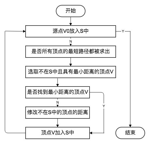
After learner modeling and clustering, to push educational resources to a specific learner, the learner is first classified, then association analysis is performed on that class’s historical learning records. The average time spent by that class of learners on each learning path in the knowledge network is computed and used as the edge weight, building a graph like the one below.
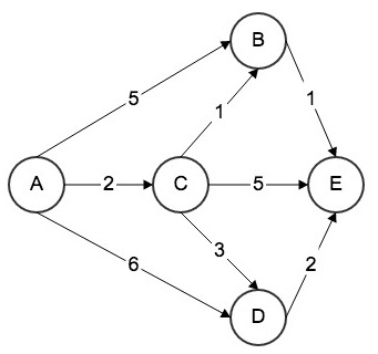
Five nodes A-E represent knowledge points; directed edges represent learning paths; edge weights represent average time units to traverse that path. For a new learner entering this network, Dijkstra’s single-source shortest path algorithm is used to recommend resources. Steps:
Step 1: Compute distances from A to directly connected nodes B, C, D:
| Destination | Path | Cost | Shortest? |
|---|---|---|---|
| B | $A \rightarrow B$ | 5 | Unknown |
| C | $A \rightarrow C$ | 2 | Yes |
| D | $A \rightarrow D$ | 6 | Unknown |
| E | Unknown | Unknown | Unknown |
Step 2: $A \rightarrow C$ is shortest (cost 2). Compute distances from C to B, D, E:
| Destination | Path | Cost | Shortest? |
|---|---|---|---|
| B | $A \rightarrow C \rightarrow B$ | 3 | Yes |
| C | $A \rightarrow C$ | 2 | Yes |
| D | $A \rightarrow C \rightarrow D$ | 5 | Unknown |
| E | $A \rightarrow C \rightarrow E$ | 7 | Unknown |
Step 3: $A \rightarrow C \rightarrow B$ < $A \rightarrow B$; shortest cost 3. Compute from B to E:
| Destination | Path | Cost | Shortest? |
|---|---|---|---|
| B | $A \rightarrow C \rightarrow B$ | 3 | Yes |
| C | $A \rightarrow C$ | 2 | Yes |
| D | $A \rightarrow C \rightarrow D$ | 5 | Unknown |
| E | $A \rightarrow C \rightarrow B \rightarrow E$ | 4 | Yes |
Step 4: $A \rightarrow C \rightarrow B \rightarrow E$ < $A \rightarrow C \rightarrow E$; shortest cost 4. E has no outgoing edges:
| Destination | Path | Cost | Shortest? |
|---|---|---|---|
| B | $A \rightarrow C \rightarrow B$ | 3 | Yes |
| C | $A \rightarrow C$ | 2 | Yes |
| D | $A \rightarrow C \rightarrow D$ | 5 | Yes |
| E | $A \rightarrow C \rightarrow B \rightarrow E$ | 4 | Yes |
The shortest path tree:
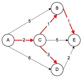
The system recommends the red path above — allowing the learner to cover all five knowledge points with minimum time and maximum efficiency.
C++ implementation of Dijkstra:
Dijkstra(Graph &graph, int s) : G(graph) {

   this->s = s;
   distTo = new Weight[G.V()];
   marked = new bool[G.V()];
   for (int i = 0; i < G.V(); i++) {
       distTo[i] = Weight();
       marked[i] = false;
       from.push_back(NULL);
   }

   IndexMinHeap<Weight> ipq(G.V());

   // start dijkstra
   distTo[s] = Weight();
   ipq.insert(s, distTo[s]);
   marked[s] = true;
   while (!ipq.isEmpty()) {
       int v = ipq.extractMinIndex();

       // distTo[v] is the shortest distance from s to v
       marked[v] = true;
       typename Graph::adjIterator adj(G, v);
       for (Edge<Weight> *e = adj.begin(); !adj.end(); e = adj.next()) {
           int w = e->other(v);
           if (!marked[w]) {
               if (from[w] == NULL || distTo[v] + e->wt() < distTo[w]) {
                   distTo[w] = distTo[v] + e->wt();
                   from[w] = e;
                   if (ipq.contain(w))
                       ipq.change(w, distTo[w]);
                   else
                       ipq.insert(w, distTo[w]);
               }
           }
       }
   }
}
Next steps involve embedding this algorithm into the intelligent learning system.